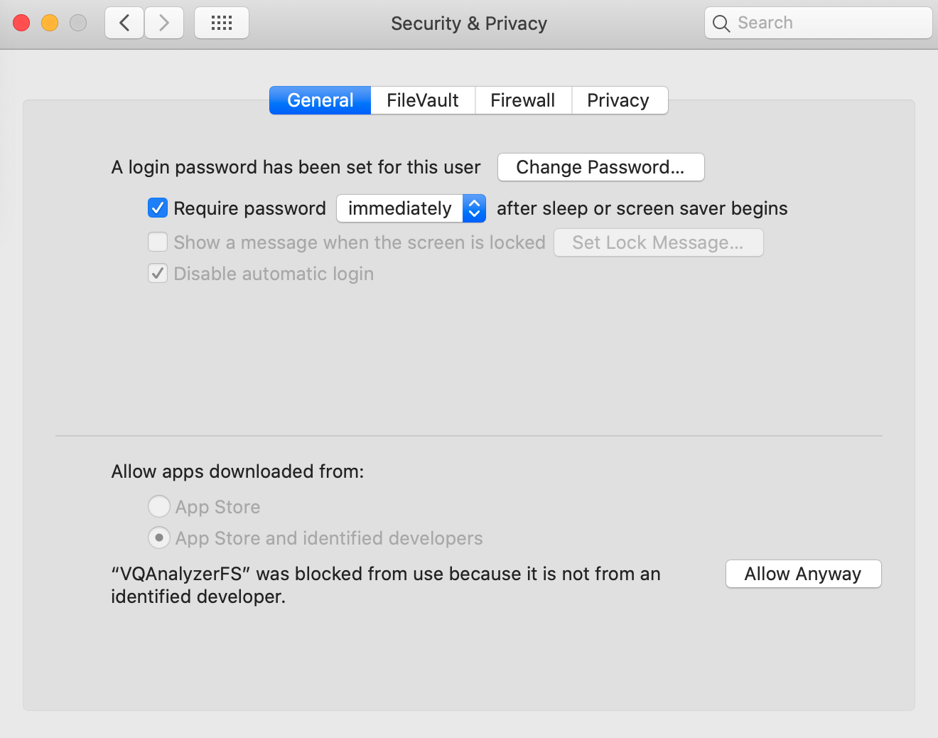
 To execute the command, you need to go to Settings -> Security & privacy, click the Allow Anyway button and execute the command again.
VQ Analyzer is a professional software tool for graphical and numerical analysis of coded video bitstreams. It supports the following video elementary streams and containers:
Elementary streams:
VQ Analyzer is written in C++. There are separate packages for each supported operation system - Windows*, Linux*, macOS*.
INFORMATION IN THIS DOCUMENT IS PROVIDED IN CONNECTION WITH VICUESOFT PRODUCTS. NO LICENSE, EXPRESS OR IMPLIED, BY ESTOPPEL OR OTHERWISE, TO ANY INTELLECTUAL PROPERTY RIGHTS IS GRANTED BY THIS DOCUMENT. EXCEPT AS PROVIDED IN VICUESOFT'S TERMS AND CONDITIONS OF SALE FOR SUCH PRODUCTS, VICUESOFT ASSUMES NO LIABILITY WHATSOEVER AND VICUESOFT DISCLAIMS ANY EXPRESS OR IMPLIED WARRANTY, RELATING TO SALE AND/OR USE OF VICUESOFT PRODUCTS INCLUDING LIABILITY OR WARRANTIES RELATING TO FITNESS FOR A PARTICULAR PURPOSE, MERCHANTABILITY, OR INFRINGEMENT OF ANY PATENT, COPYRIGHT OR OTHER INTELLECTUAL PROPERTY RIGHT.
UNLESS OTHERWISE AGREED IN WRITING BY VICUESOFT, THE VICUESOFT PRODUCTS ARE NEITHER DESIGNED NOR INTENDED FOR ANY APPLICATION IN WHICH THE FAILURE OF THE VICUESOFT PRODUCT COULD CREATE A SITUATION WHERE PERSONAL INJURY OR DEATH MAY OCCUR.
VICUESOFT may make changes to specifications and product descriptions at any time, without notice. Designers must not rely on the absence or characteristics of any feature or instruction marked "reserved" or "undefined." VICUESOFT reserves these for future definitions and holds no responsibility for conflicts or incompatibilities arising out of future changes to them. The information here is subject to change without notice. Do not finalize a design with this information.
The products described in this document may contain design defects or errors known as errata which may cause the product to deviate from published specifications. Current characterized errata are available on request.
Contact your local VICUESOFT sales office or distributor to obtain the latest specifications before placing your product order.
MPEG is an international standard for video compression/decompression promoted by ISO. Implementations of MPEG CODECs, or MPEG enabled platforms may require licenses from various entities, including VICUESOFT.
*Other names and brands may be claimed as the property of others.
Copyright © 2017-2026, VICUESOFT Ltd. All Rights reserved.
VQ Analyzer User Manual describes the main functionality and GUI of the tool. It has the following structure:
Introduction overviews the product, describes product activation process and command line features;
UI Components part describes Main Menu, Main Panel, Stream View, Syntax Info (codec-specific), Selection Info (codec-specific), Unit Info, HEX View, and Status panel;
Modes part describes modes according to specific codecs;
Global functions part describes functions common to all codecs - Dual View, Run full stream analysis, Debug YUV;
The Miscellaneous and Attributions parts describe additional information on the product and attributions.
| Term/Abbreviation | Definition |
|---|---|
| AV1 | open, royalty-free video coding format developed by the Alliance for Open Media |
| AVC | Advanced Video Coding |
| AVS3 | AVS3 video coding standard - third generation standard developed by China AVS working group |
| CABAC | Context-adaptive binary arithmetic coding |
| CTB | Coding Tree Block |
| CU | Coding Unit |
| CVS | Coded Video Stream |
| GUI/UI | (Graphical) User Interface |
| HEVC | High Efficiency Video Coding |
| MPEG2 | ISO/IEC 13818-2 / ITU-T Rec. H.262 coding standard |
| NAL | Network Abstraction Layer |
| OBU | Open Bitstream Unit |
| PPS | Picture Parameter Set |
| PU | Prediction Unit |
| QM | Quantization Matrix |
| SAO | Sample adaptive offset |
| SB | SuperBlock |
| SEI | Supplemental Enhancement Information |
| SPS | Sequence Parameter Set |
| TU | Transform Unit |
| VP9 | open and royalty free video coding format developed by Google |
| VPS | Video Parameter Set |
| VVC | Versatile Video Coding (MPEG-I Part 3) video compression standard |
| YUV | Color space (YUV) |
The VQ Analyzer supports several modes of working, depending on the activation information supplied by the user.
If you are running the VQ Analyzer for the first time on the machine licensing system, the license server will connect (over the internet) to register itself and activate the verified trial mode. In this mode you have a trial period to evaluate the product. The only restriction you have is a splash screen that will appear every 5 minutes to remind you that you're in evaluation mode. There is a grace period of several days during which application can run without internet connection. The verified trial period can be extended by entering the special serial number in the Product run without internet connection. Verified trial period can be extended through the activation dialog. The number of remaining days can be checked in the 'About' menu.
If you don't have internet connection or if the verified trial is over, the application runs in pure trial mode, whereby you can load only sample streams provided in the package.
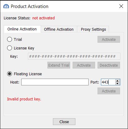
If you have a single user license and serial number you have to enter them in the 'Activate' dialog under 'Help' menu. In the 'Online Activation' tab, enter your serial number in the 'Key' line and click 'Activate'. If you check 'Extend Trial', the serial number will be used to extend the verified trial.
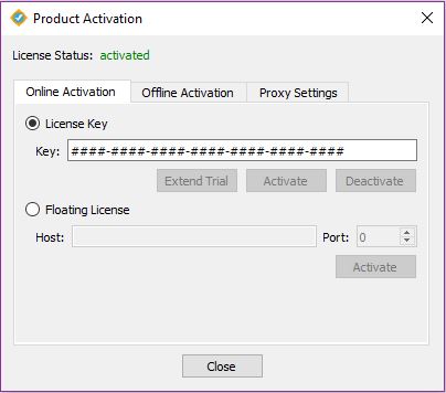
If that application is already activated, the 'Deactivate' button will be shown instead of the 'Activate' button. You are then able to deactivate the application on this computer, and reactivate it later, on another or the same computer, as many times as is allowed by your license.
If you have a floating license you have to install the floating server in your network and enter the host and port for it in the 'Activate' dialog under the 'Help' menu after checking the 'Floating License' option.
Also you have the opportunity for Offline Activation. Open the 'Activate' dialog under the 'Help' menu and choose the 'Offline Activation' tab. Follow the instructions.
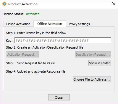
First, enter your serial number in the 'Key' line. Press 'Activation Request' button if you want to activate this application, or click the 'Deactivation Request' button if you need to deactivate it. Choose the directory for saving the Request file, then click 'Show in folder', find your Request file and send it to [email protected]. You will receive a response after a short time. The last step is to upload the Response file in the 'Offline Activation' tab.
Any choice of parameters in the 'Activate' dialog are stored in the system settings and used for both GUI and command line versions.
The same procedures can also be done with the command line tool:
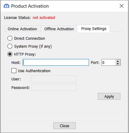
The VQ Analyzer can be configured to work behind a firewall. Currently, http/https proxies are supported. Normally, proxy settings are detected based on system settings and you don't need to change them. But if the system settings are wrong or you prefer to use other proxy connection type, you will have to set up the required setting in the 'File -\> Proxy settings' dialog.
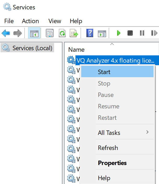
To activate FS via proxy server:
On premise FS installation is NOT allowed on virtual machine, make sure it shall be a bare metal computer to host FS. Customers on Premium Support May delegate FS hosting to VICUESOFT cloud
To perform the following commands, you would need to have the Administrator’s rights (sudo). When performing commands containing sudo, you will be asked for the password which you will have to enter into the terminal.
chmod +x ~/vicue_float_server_lin/VQAnalyzerFSThis command gives the right for executing VQAnalyzerFS file
Activation can be performed either online (Step 2.1) or offline (Step 2.2).
Enter the following command into the terminal:
sudo ~/vicue_float_server_lin/VQAnalyzerFS -a=YOUR-LICENSE-KEYAfter performing this command you should receive notification of the successful activation "Activated successfully"
sudo ~/vicue_float_server_lin/VQAnalyzerFS -a=YOUR-LICENSE-KEY -areq="/home/USER_NAME/Documents/ActivationRequest.xml"sudo ~/vicue_float_server_lin/VQAnalyzerFS -a=YOUR-LICENSE-KEY -aresp="/Location/to/File/ActivationResponse.xml"After performing this command you should receive notification of the successful activation "Activated successfully"
To launch the server, enter the command into the terminal:
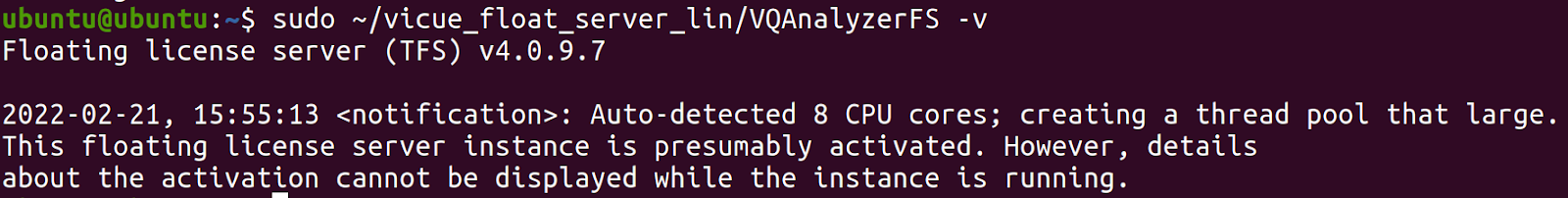
sudo ~/vicue_float_server_lin/VQAnalyzerFS -x -silentCongratulations! The server is now activated and launched. Below there are some additional commands which can be useful for acquiring information on FS.
Enter the following command into the terminal:
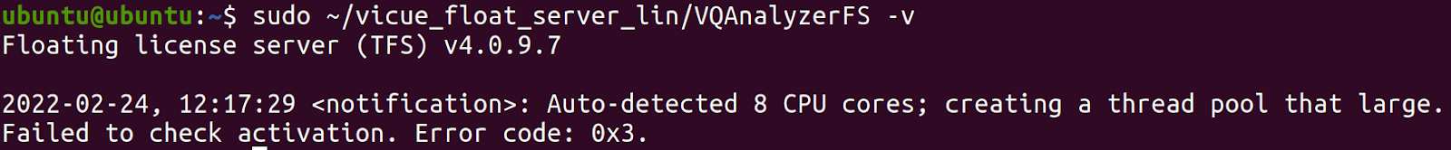
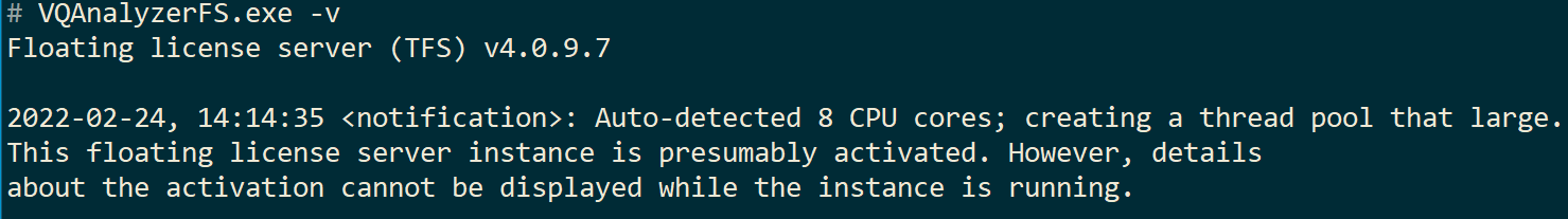
sudo ~/vicue_float_server_lin/VQAnalyzerFS -v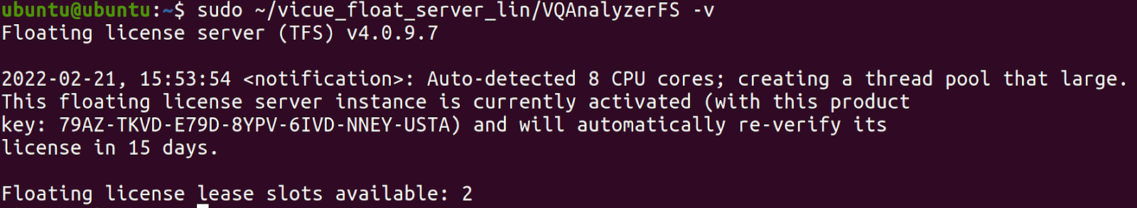
Enter the following command into the terminal:
ps aux | grep VQAnalyzerFSYou will receive information about the launched FS processes.

pidof VQAnalyzerFSYou will receive PID of the process
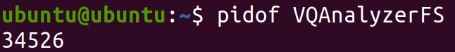
sudo kill 34526(This is PID of the process which will displayed after entering the previous command)
Enter the following command into the terminal:
sudo ~/vicue_float_server_lin/VQAnalyzerFS -x -silentsudo ~/vicue_float_server_lin/VQAnalyzerFS -deactYou will receive notification of the successful deactivation: "Deactivated successfully"
sudo ~/vicue_float_server_lin/VQAnalyzerFS -deact="/home/USER_NAME/Documents/DeacivationRequest.xml"To perform the following commands, you would need to have the Administrator’s rights.
cd C:\vicue_float_server_win\Activation can be performed either online (Step 2.1) or offline (Step 2.2).
Enter the following command into the command line:
VQAnalyzerFS.exe -a=YOUR-LICENSE-KEYAfter performing this command you should receive notification of the successful activation "Activated successfully".
VQAnalyzerFS.exe -a=YOUR-LICENSE-KEY -areq="C:\Users\USER_NAME\Documents\ActivationRequest.xml"VQAnalyzerFS.exe -a=YOUR-LICENSE-KEY -aresp="C:\Users\USER_NAME\Downloads\ActivationResponse.xml"After performing this command you should receive notification of the successful activation "Activated successfully".
To install and launch the server, enter the command into the command line:
VQAnalyzerFS.exe -iAfter performing this command you should receive notification of the successful installation "Service installed successfully".
Congratulations! The server is now activated and launched. \nBelow there are some additional commands which can be useful for acquiring information on FS.
Enter the following command into the command line:
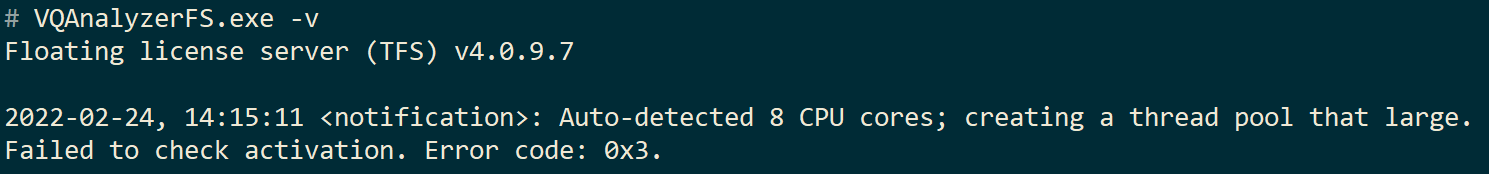
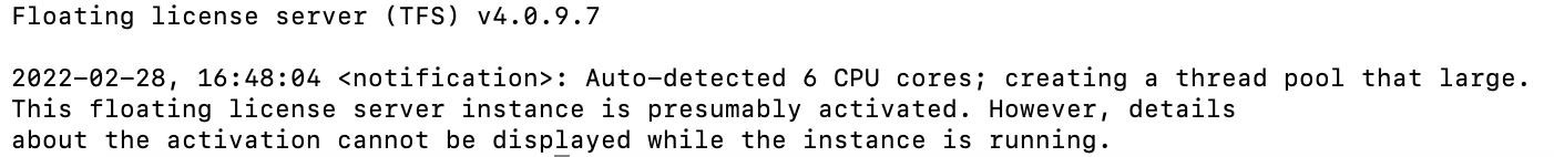
VQAnalyzerFS.exe -v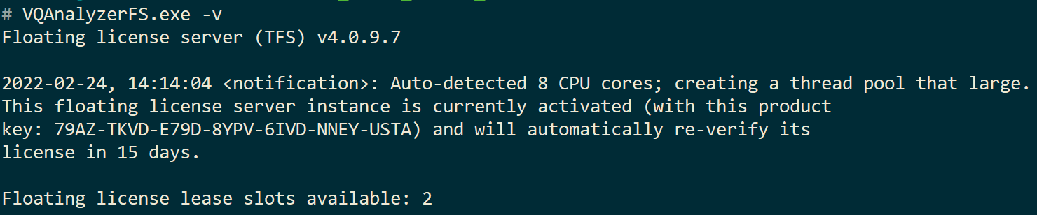
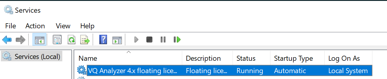
Empty Status signals about stopped FS.
Status "Running" signals about running FS. (indicates that the server is running)
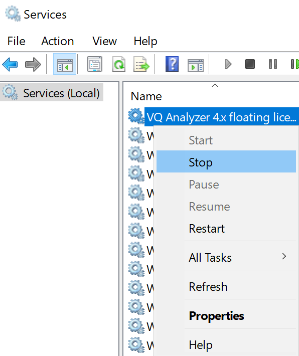
VQAnalyzerFS.exe -deactYou will receive notification of the successful deactivation: "Deactivated successfully"
VQAnalyzerFS.exe -deact="C:\Users\user_name\Documents\DeacivationRequest.xml"After performing this command, the server will be deactivated. A file will be created which needs to be sent to [email protected]
To perform the following commands, you would need to have the Administrator’s rights (sudo). When performing commands containing sudo, you will be asked for the password which you will have to enter into the terminal. There are two ways: recommended and not recommended. If necessary, there will be a division into these ways in sections.
chmod +x ~/Documents/vicue_float_server_mac/VQAnalyzerFSThis command gives the right for executing VQAnalyzerFS file
Activation can be performed either online (Step 2.1) or offline (Step 2.2).
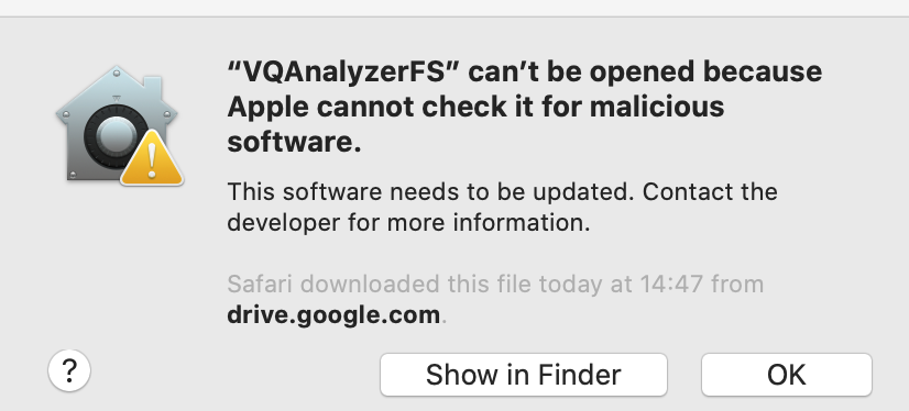
You may receive a warning while the command is executing.
To execute the command, you need to go to Settings -> Security & privacy, click the Allow Anyway button and execute the command again.
Enter the following command into the terminal:
sudo ~/Documents/vicue_float_server_mac/VQAnalyzerFS -a=YOUR-LICENSE-KEYAfter performing this command you should receive notification of the successful activation "Activated successfully"
sudo ~/Documents/vicue_float_server_mac/VQAnalyzerFS -a=YOUR-LICENSE-KEY -areq="/Users/USER_NAME/Documents/ActivationRequest.xml"sudo ~/Documents/vicue_float_server_mac/VQAnalyzerFS -a=YOUR-LICENSE-KEY -aresp="/Location/to/File/ActivationResponse.xml"After performing this command you should receive notification of the successful activation "Activated successfully"
Recommended way:
sudo ~/Documents/vicue_float_server_mac/VQAnalyzerFS -x -silentNot recommended way:
sudo ~/Documents/vicue_float_server_mac/VQAnalyzerFS -i**Congratulations! The server is now activated and launched. Below there are some additional commands which can be useful for acquiring information on FS.**
Enter the following command into the terminal:
sudo ~/Documents/vicue_float_server_mac/VQAnalyzerFS -v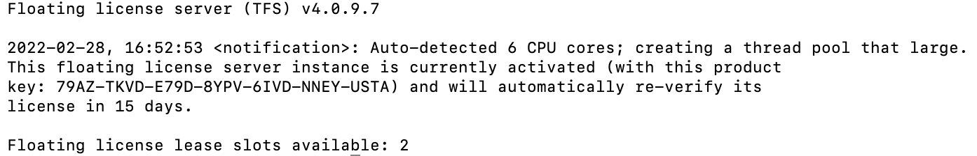

Enter the following command into the terminal:
ps aux | grep VQAnalyzerFSYou will receive information about the launched FS processes.

Note: The second column contains the process id. In this example process id is 129. It may be necessary to stop FS.
Recommended way:
-x or -x -silent arguments, then the active process in the terminal must be terminated. (Interrupting in the terminal can be done with the combination Ctrl+C).sudo kill idNot recommended way:
sudo launchctl list | grep turboYou will receive full name of the proccess

sudo launchctl stop com.turbofloatserver.4449(This is full name of the process which will displayed after entering the previous command)
You must have the server turned off.
Recommended way:
sudo ~/Documents/vicue_float_server_mac/VQAnalyzerFS -x -silentNot recommended way:
sudo ~/Documents/vicue_float_server_mac/VQAnalyzerFS -deactYou will receive notification of the successful deactivation: "Deactivated successfully"
If you receive a notification: "You can only run one instance of this floating license server at a time". It means that the server is not stopped. Please use the notes from the sections Testing FS launch and How to stop FS.
sudo ~/Documents/vicue_float_server_mac/VQAnalyzerFS -deact="/Users/USER_NAME/Documents/DeacivationRequest.xml"
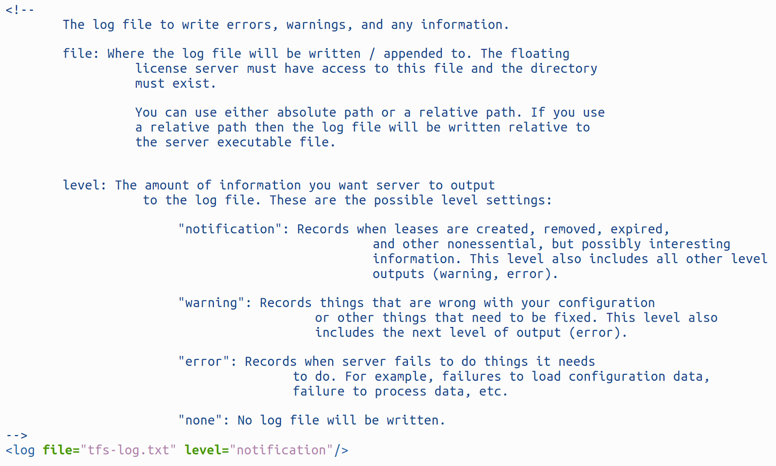
Possible level settings:
To completely uninstall the VQ Analyzer, follow these steps below:
If the cache cleanup is successful, you will see the following message: VQ Analyzer has been successfully uninstalled.
If the cache cleanup is successful, VQ Analyzer will be fully removed from the system.
Important: Before starting, make sure Terminal has Full Disk Access.
If the cache cleanup is completed successfully, the following message will appear in Terminal: VQ Analyzer has been successfully uninstalled.
Warning: after all of the previous or current version's settings, including the license key, will be deleted from the system.
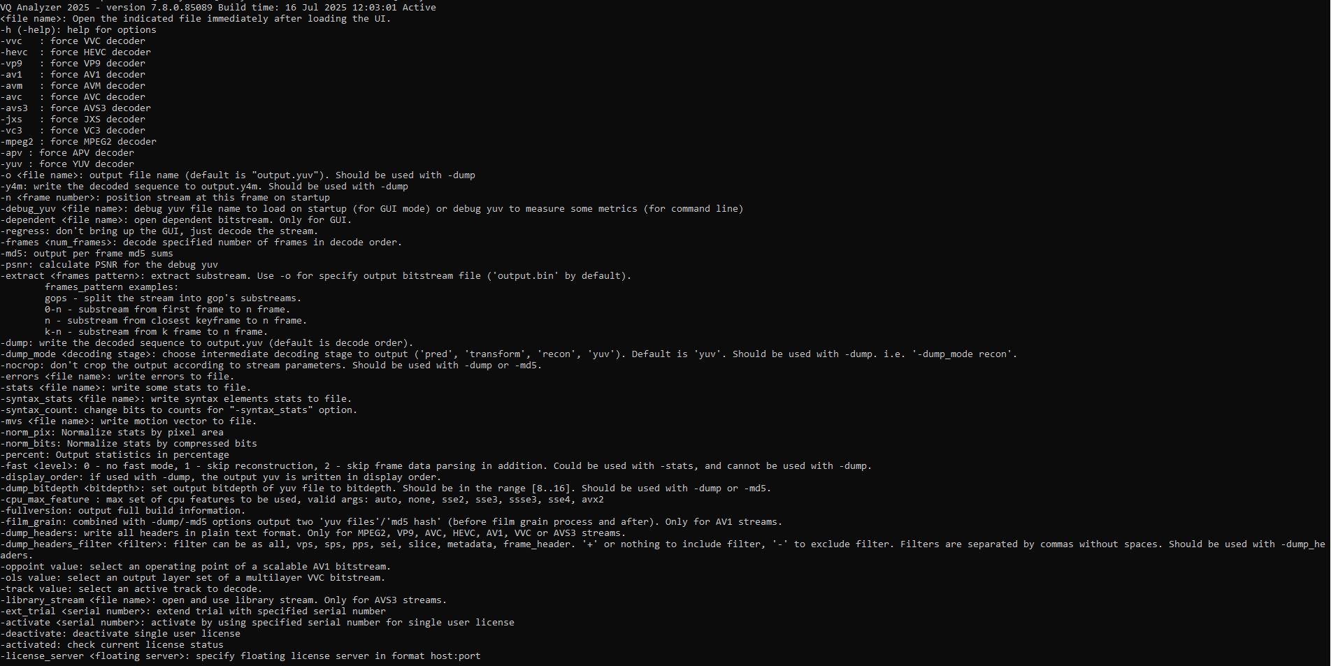
VQ Analyzer has a separate console application in Windows* to run in command line mode. The GUI application in Windows* also accepts the same command line options but does not provide console output.
VQ Analyzer has the following command line options:
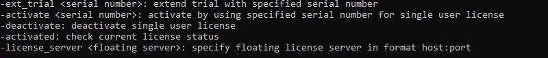
<file name>: output file name (default is "output.yuv"). Must be used with -dump<frame number>: position stream at this frame on startup<file name>: debug yuv file name to load on startup (for GUI mode) or debug yuv to measure some metrics (for command line)<file name>: open dependent bitstream. Only for GUI<num_frames>: decode specified number of frames in decode order.<frames pattern>: extract substream. Use -o for specify output bitstream file ('output bin' by default).<decoding stage>: choose intermediate decoding stage to output ('pred', 'transform', 'recon', 'yuv'). Default is 'yuv'. Should be used with -dump. i.e. '-dump_mode recon'.<file name>: write errors to file.<file name>: write some stats to file.<file name>: write syntax elements stats to file.<level>: 0 - no fast mode, 1 - skip reconstruction, 2 - skip frame data parsing in addition. Could be used with -stats, and cannot be used with -dump.<bitdepth>: set output bitdepth of yuv file to bitdepth. Should be in the range [8..16]. Should be used with -dump or md5.<filter>: filter can be as all, vps, sps, pps, sei, slice, metadata, frame_header. '+' or nothing to include filter, '-' to exclude filter. Filters are separated by commas without spaces. Should be used with -dump_headers.<file name>: open and use library stream. Only for AVS3 streams.<serial number>: extend trial with specified serial number<serial number>: activate by using specified serial number for single user license<floating server>: specify floating license server in format host:portThe following sections describe the UI components when a bitstream is loaded.
Main menu has the tabs File, Mode, YUVDiff, Options, View, Help. They are described below.
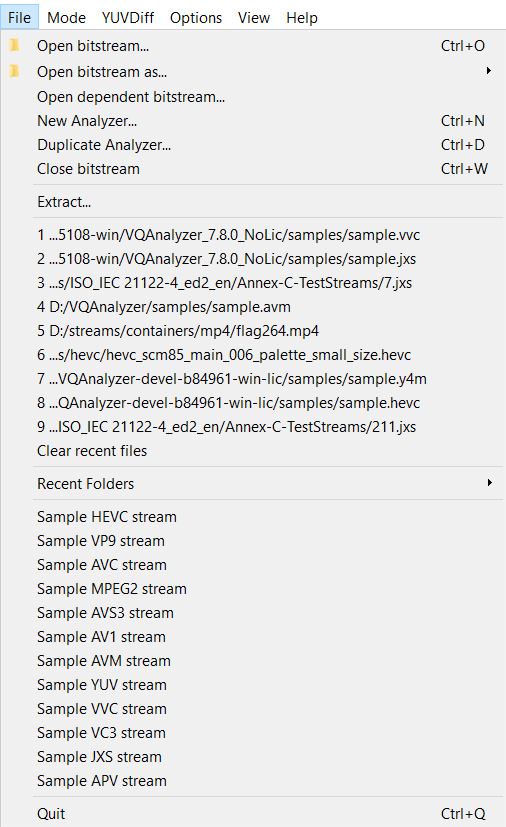
File menu allows the user to operate with bitstream files.
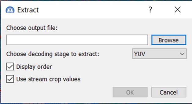
Once the Extract dialogue window is open, enter the output file name and its location or choose the output file by clicking on Browse. Then choose decoding stage to extract from YUV, Prediction, Transform and Reconstruction. Tick or untick Display order and Use stream crop values. Press OK to proceed.
File menu can also open sample codec bitstreams – MPEG, AVC, HEVC, VP9, AV1, VVC, AVS3, YUV.
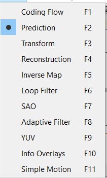
With a bitstream loaded, VQ Analyzer can be put into one of available modes using either Mode menu or F1-F12 keys. The selection of modes is specific to each codec and is described in detail in the relevant section of Modes.
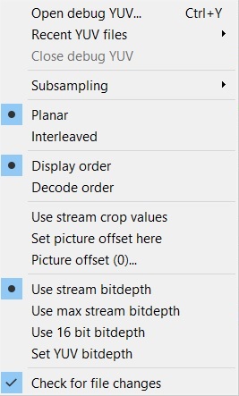
YUVDiff menu allows to operate with YUV files.
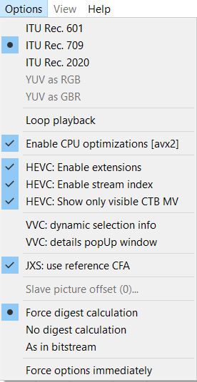
Options menu allows the user to choose between different types of operation modes. The first options switch between ITU Rec. 601, ITU Rec. 709 and ITU Rec. 2020 color conversion standards, used to map YUV data on an RGB surface. VQ Analyzer uses the chosen type of YUV conversion on its next picture conversion. Conversions that have already been completed will remain unchanged.
For specific coding modes, like HEVC screen content coding, two additional modes can be used: "YUV as RGB" and "YUV as BGR". In this case, decoded YUV values are directly mapped onto RGB or BGR values for monitoring.
Color conversion can be achieved with the following transformation (0.0 <= [Y,R,G,B] <= 1.0) ; (-1.0 < [U,V] < 1.0)), where Y,U,V are normalized accordingly:
R = Y + V*(1-Kr)\ G = Y - U*(1-Kb)*Kb/Kg - V*(1-Kr)*Kr/Kg\ B = Y + U*(1-Kb),
Where Kr, Kb, Kg have the following values:
| Kr | Kg | Kb | |
|---|---|---|---|
| ITU Rec. 601 | 0.299 | 0.587 | 0.114 |
| ITU Rec. 709 | 0.2126 | 0.7152 | 0.0722 |
| ITU Rec. 2020 | 0.2627 | 0.6780 | 0.0593 |
View Menu turns on/off main UI components – Stream View, Selection Info, Unit Info, Status, Syntax Info. For detailed description of these panels see corresponding sections in UI Components.
Help Menu has the following options:
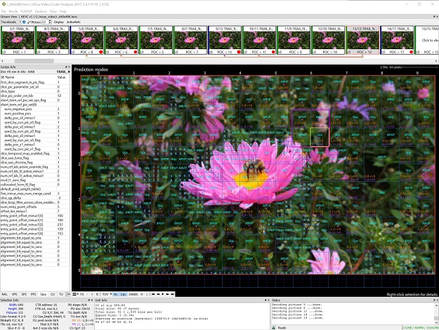
The main panel displays the selected picture with visual annotations. The type of annotations and associated interactive behavior depends on the current mode. Clicking and dragging moves the picture around, and the mouse wheel zooms in or out around the mouse cursor.
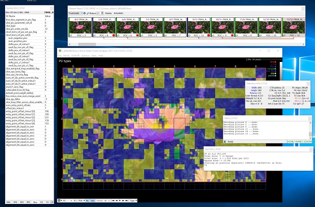
At the top left of the panel, the current mode is displayed. Along the top right the current scale is shown. In all modes, the CTB row and column values are displayed along the left and top border of the picture, slices are indicated with thick red lines, dependent slice boundaries are dashed red lines and tile boundaries are thick green lines. The screenshot above shows an example of a stream that is 13x8 CTBs, has 6 tiles and a number of slice segments, some of which are dependent. The selected CU is outlined with a pink box.t mode and is displayed. Along the top right the current scale is shown. In all modes, the CTB row and column values are displayed along the left and top border of the picture, slices are indicated with thick red lines, dependent slice boundaries are dashed red lines and tile boundaries are thick green lines. The screenshot above shows an example of a stream that is 13x8 CTBs, has 6 tiles and a number of slice segments, some of which are dependent. The selected CU is outlined with a pink box.
The information in the top right corner shows the current zoom factor and pixel length at selected zoom. By double clicking on zoom factor you can reset it to 1x factor.
The mode selection affects only what is displayed in the Main Panel. Most modes can also show details of the current selection (CU, MB ...) . This can be toggled with the right mouse button or the main panel's button strip.
The bottom left side has a cluster of buttons:

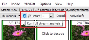
When you click "Run full stream analysis" the VQ Analyzer performs the following for all codecs:
And for HEVC codec it:
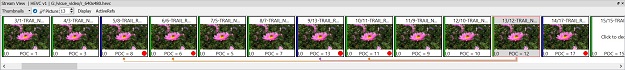
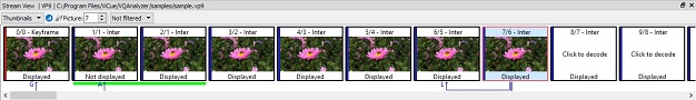
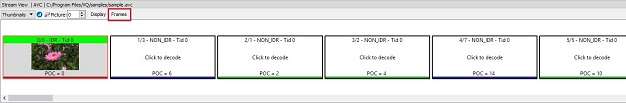
The top filmstrip is a horizontally scrolling overview of the pictures in the bitstream. The current picture is highlighted. When a new sequence begins, the top info label is highlighted in green. The current picture is highlighted with a red border. On top is the frame number in decode and display order respectively, and the picture type/structure as indicated by the frame header. Or there is the picture number - the decode order index in the bitstream - and the first slice in the picture type as indicated by the NAL unit types. On the bottom there is the layerId, shown as Lx where is x gives the layerId itself, and the POC value or indicated if the picture should be displayed or not. Referenced pictures for the current picture are indicated with arrows. Green arrows indicate the long-term references. The bar filmstrip has an underlining green band under those frames that begin new CVS. Picture type is colour coded: red – intra picture (I), blue – P-picture, green – B-picture. Red dots show how often the picture is used as a reference picture. The size of the dot is proportional to this usage index. By using this information, you can get an idea which image is most important in predicting other images.
The title bar shows the currently loaded stream and the selected codec for it. Clicking on a picture will cause the VQ Analyzer to decode it and mark it as the current picture, updating the rest of the UI correspondingly. If the new picture requires other pictures to be available as reference that have not yet been decoded, those will automatically be decoded.
Pictures are decoded on demand since it is impractical to store all details of all pictures in memory, especially for HD sequences. The current picture can also be selected by typing in the picture number in the box on the left of the panel. When using this box, the filmstrip is scrolled in such a way that the newly selected current picture is visible.
When a frame from the IVF or WebM/MKV container is a super frame (meaning 1 or more non-displayed picture and one displayable), this collection of pictures has superscription with a line over the frames belonging to the super frame. The bar filmstrip has an underlining green band under the frames belonging to the same super frame.
The application title bar shows the currently loaded stream, its selected codec and the process ID for easier identification of dock widgets. When any dock widget is detached from the main window, its title bar will also show the process ID of the main window.
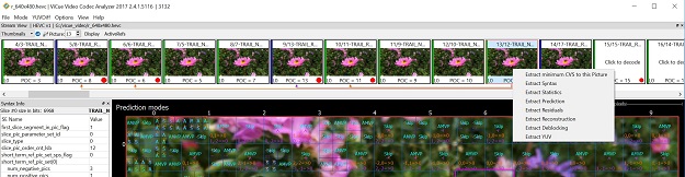
By right-clicking on the selected picture you can see a popup submenu with a set of extract actions. An action called "Extract minimum CVS to this Picture" (HEVC spec.) will write out a bitstream that contains the minimum number of pictures needed to decode the current picture. Typically, this will consist of the current picture and all previous pictures that are reference pictures up to the nearest IRAP picture. This can be useful for debugging any issues in long sequences. For other codecs this action may be called "Extract pictures form last keyframe to the Picture" or "Extract pictures from last IDR to the Picture". Other actions allow you to save in the output file statistics and intermediate/final YUV planes. For VC3 bitstreams of RGB(A) format Extract Packed RGB action is availanbe.
All separate panels can be detached from the main window or hidden. To reattach panels then, double click on the titlebar. To unhide a panel go to the View menu and select the appropriate panel.
There are a set of extended modes that can be accessed via menus in the Stream View toolbar. In the Thumbnails and Bar mode it is possible to choose between Display/Decode order representation with an additional click.
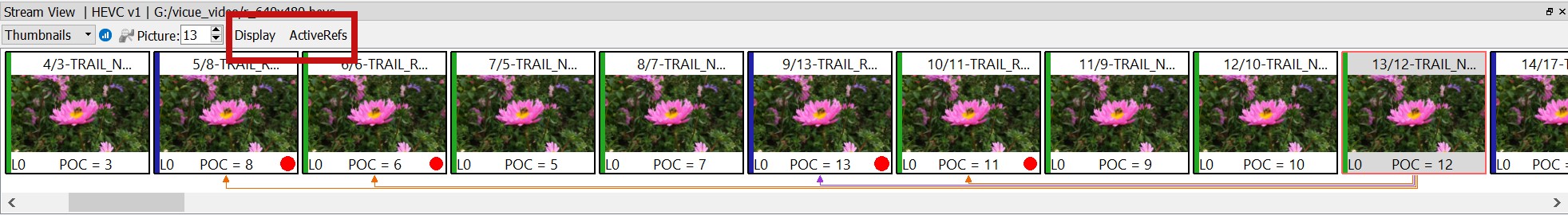
There are three possible modes with two sub-modes that can then be selected. Sub-modes of the currently selected mode change dynamically depending on the current mode.
Using the filter, you can hide the “Not displayed” frames.
The field option gives special visualization capabilities for streaming with fields. Namely, it shows references on a per-field basis. The VQ Analyzer shows the top and bottom fields as they occur in the stream. Their position is shifted according to whether the top or bottom flag is used for the field.
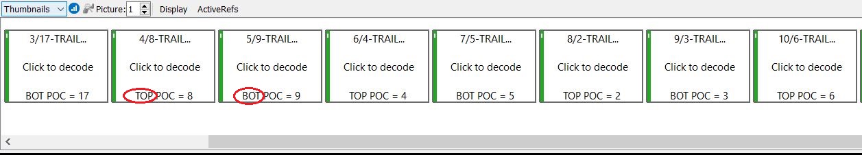
In VVC bitstreams coded by fields each field is shown in thumbnails as frame indicating TOP or BOT (for bottom field) on it in display or decode order. Console analyzer glues the fields in the resulting YUV file.
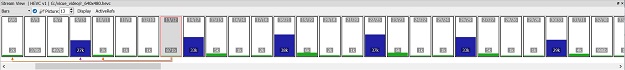
All supported codecs have Frame sizes view. When you choose the "Buffer" menu from popup toolbar, the frame sizes view will appear by default. This is a bar chart, plotted with frame sizes. Each bar is colored according to the frame type. When you move the mouse along the bar, the current frame is highlighted and the tooltip shows information about the current frame. By clicking on the selected frame you can decode it. When you press the left mouse button and drag, all plots move along both axes. You can zoom in and out with mouse wheel on both axis when the cursor is inside the canvas. Reset plot button in context menu resets the plot back to default settings. If the mouse is to the left or below the main x and y axes you can zoom, pan or double click only on one axis (for example, keep the cursor to below the main chart to alter only the x-axis). All actions will then only be applied to that axis.
The movement of the plots is restricted to positive values only, so you can't move or zoom in a negative direction. The currently decoded frame is shown with a vertical line and the frame number on it.
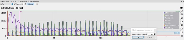
On the right axis, the average slice QP values are shown. When full stream analysis is complete, the VQ Analyzer adds average block QP plot that is also attached to the right axis. By double clicking on the 'Moving average' label item, the sliding window size can be adjusted in the separate dialog.
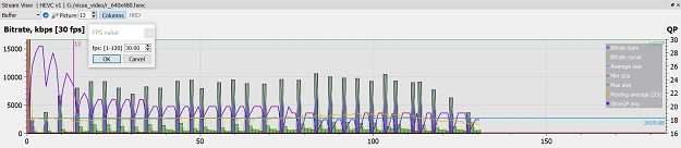
By double clicking on the '[30fps]' label item, the fps value can be adjusted in the separate dialogue box. Clicking on the legend item dialogue can switch it on and off. The legend panel can also be moved by clicking and dragging.
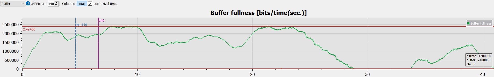
The “HRD” sub-mode is enabled if a stream has HRD parameters in it, otherwise it is disabled (greyed out).
Blue dashed line shows final arrival time of picture.
General HRD mode (check box is unchecked) builds plot using information only about bitrate and removal time of pictures. So if any gaps between current picture earliest arrival time and previous picture final arrival time exit, then plot can be a little bit wrong. HRD mode with arrival times (check box is checked) builds plot using all available times and inserts points on initial arraival time, final arraival time and on removal time. Navigation is anchored by picture removal time in any mode (so we see rose line at removal picture time (this picture is decoded) and blue dashed line on its picture final arrival time).
A right-click on the central area of the plot in the VQ Analyzer shows additional options for plot adjustment. In this same popup menu you can export HRD timings into a .csv file.
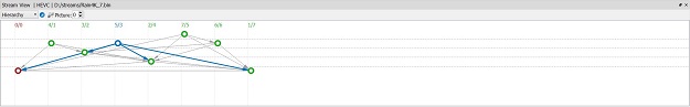
The VQ Analyzer shows B-pyramid visualization when the Hierarchy in the Stream View option is selected. It shows the level of mutual B-frame references, frame numbers in decoding /display orders, frame type coded by color and frame references. By clicking on each frame you can highlight particular frame references.
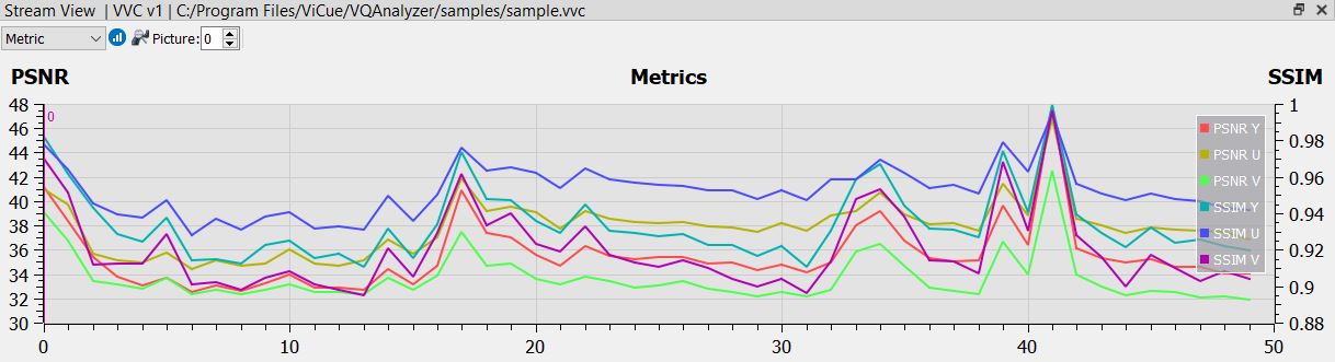
The analyzer displays PSNR and SSIM plots for each component - one for luma (Y) and two for chroma (U and V). To display the plots, load the debug YUV file and run a full stream analysis by clicking on 'Run full stream analysis' button. To hide the plot, click on the corresponding legend.
Syntax Info panel is to the left side of the UI. It is a resizable panel with several tabs displaying information about the current selection. The following subsections describe tabs according to codecs.
Syntax Info panel can be switched on/off by ticking/unticking Syntax Info in View in Main menu. When switched on, it is displayed in the left side of the UI as a resizable panel with several tabs located at its bottom. The tabs display information about the syntax of the selected picture and the stream (see Stream View panel description). Bringing the mouse to the tab name shows explanation of its abbreviated name. The following subsections describe each tab in Syntax Info panel.
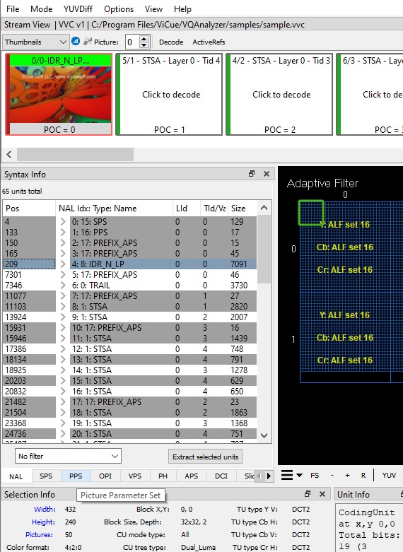
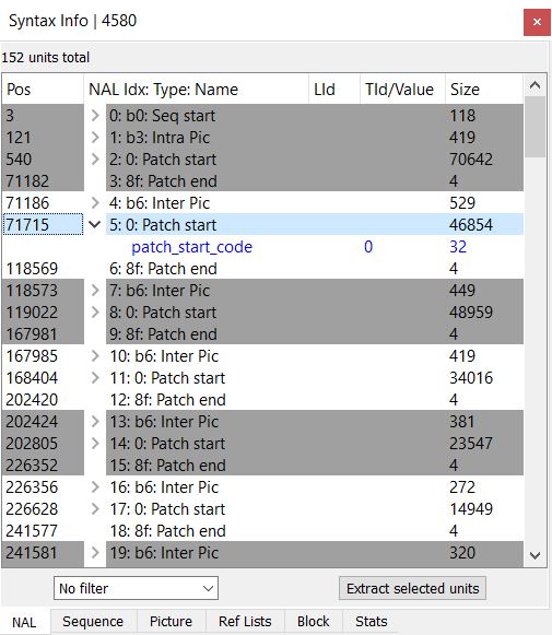
NAL (Network Abstraction Layer Units) tab displays a table with all units in the bitstream in decode order.
Above the list of the units the total number of units is displayed. The table has the following columns:
Pos - byte position of the unit in the file,
NAL Idx: Type: Name - NAL's index, type, name,
LId - Layer ID of the unit,
Tld/Value - Temporal ID of the unit/value of syntax element
Size - total number of bytes in the unit.
The unit descriptions are colored white or gray in blocks. Units in each block belong to one picture. Therefore, a change in color indicates a picture border.
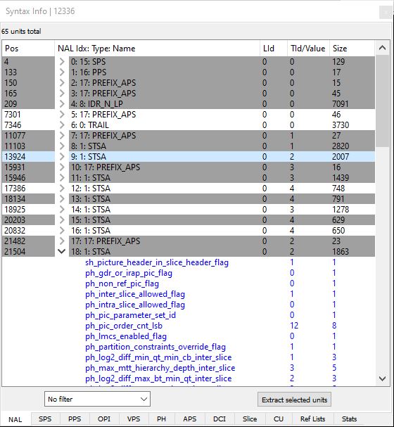
In the second column, for some units there is a branch sign. Clicking on it, rolls out unit syntax elements as read from the bitstream. For each syntax element, VQ Analyzer shows its value and the number of bits it occupies in the bitstream. Red elements signal an error syntax element.
Clicking on any unit will display information on raw bytes of the unit in Unit Info panel. (For this, Unit Info panel needs to be switched on in View in Main panel.) Unit Info tab will show up to the first 500 raw bytes of the unit. Hex View Tab will highlight in yellow all raw bytes belonging to this unit.
Any unit can be double-clicked in order to bring forward the picture it belongs to as the current picture in Stream View and Main panel. Selecting a block in the Main panel will highlight the unit containing the slice with the selected block in NAL tab.
At the bottom of the unit tab is a button called Extract selected units. Clicking this button will write all the selected units out to a file.
At the bottom of the unit tab there also a combo box which allows to select or filter the units in the list. By default it is set to No Filter.
SPS (Sequence Parameter Set) tab shows all syntax elements (SE) decoded in the sequence header and sequence extension header with values.
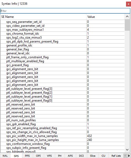
Hovering the mouse over the name of the syntax element brings up a window with its description from the codec specification.
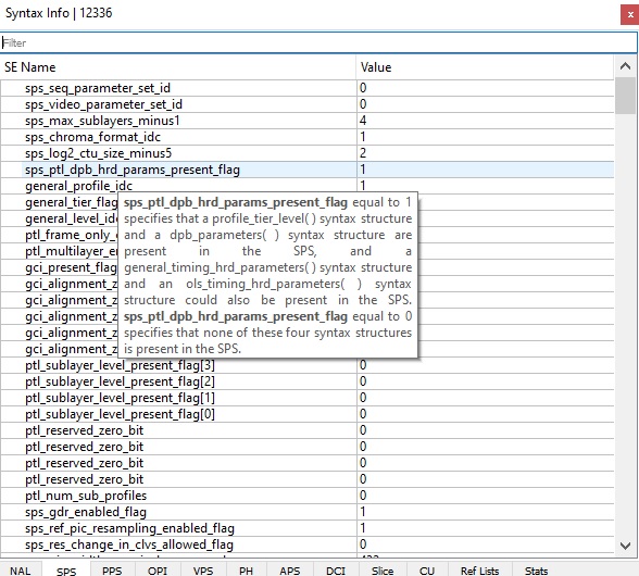
Right-clicking the mouse opens up a context menu with the following functionality:
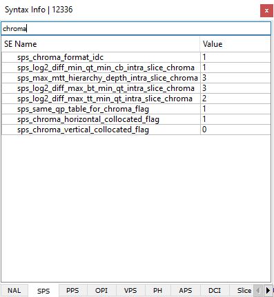
Filter box allows to search for a SE by its name.
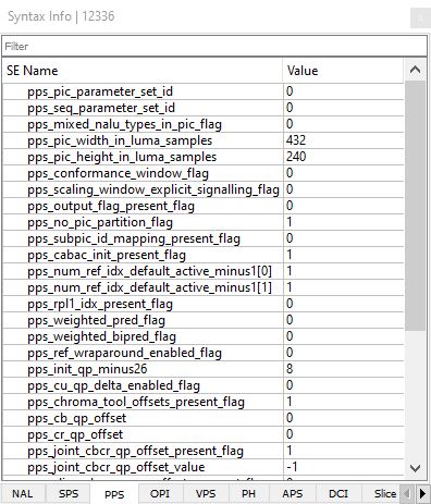
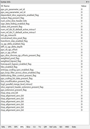
PPS (Picture Parameter Set) tab shows all syntax elements decoded in the picture header, picture coding extension, picture display extension and picture spatial scalable extension with values.
Hovering the mouse over the name of the syntax element brings up a window with its description from the codec specification.
Right-clicking the mouse opens up a context menu with the following functionality:
Filter box allows to search for a SE by its name.
TBD
TBD
TBD
APS (Adaptation Parameter Set) tab shows syntax elements that apply to zero or more slices as determined by zero or more syntax elements found in slice headers with their values.
Hovering the mouse over the name of the syntax element brings up a window with its description from the codec specification.
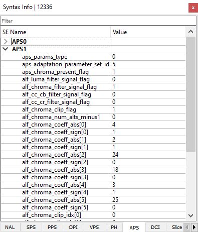
Right-clicking the mouse opens up a context menu with the following functionality:
Filter box allows to search for a SE by its name.
TBD
Slice tab shows all syntax elements decoded in the slice header with values.
At the top, the size of the slice is given in bits.
Hovering the mouse over the name of the syntax element brings up a window with its description from the codec specification.
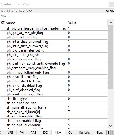
Right-clicking the mouse opens up a context menu with the following functionality:
Filter box allows to search for a SE by its name.
CU (Selected Coding Unit Syntax) tab contains a list of the decoded syntax elements of the currently selected CU in the Main Panel. For this information to be displayed, a block needs to be highlighted by clicking the left button of the mouse in Main view. Continuous clicking on the unit expands the highlighted area in the hierarchy up to the CTU. The relevant information is displayed in the table according to the level highlighted. The table lists the following parameters: PoS, R, V, SE Name, Value, Bits, Bits %.
Hovering the mouse over the name of the syntax element brings up a window with its description from the codec specification.
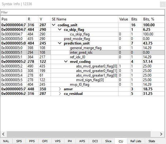
Right-clicking the mouse opens up a context menu with the following functionality:
Filter box allows to search for a SE by its name.
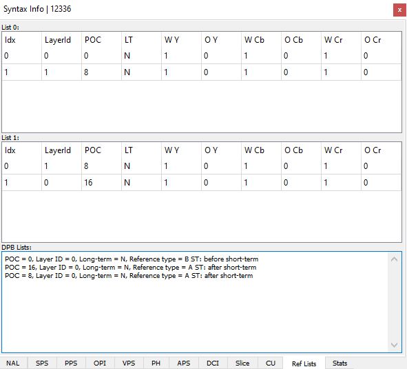
Ref Lists (Reference Lists) tab displays details of reference lists L0 and L1, as well as DPB Lists. L0 and L1 lists have the following columns:
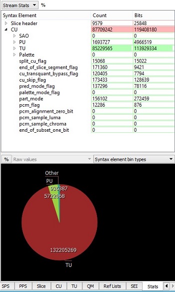
Stats (Statistics) tab displays various types of statistics in the bitstream, namely picture statistics, per syntax element statistics, and overall stream statistics. This panel has two parts - top and bottom.
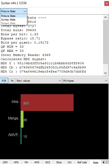
The top part gives an option of selecting between Picture Stats, Syntax Stats, and Stream Stats **in the combo box. **Picture Stats gives picture statistics, compression statistics as well as the image digest information.
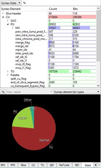
Syntax Stats lists Counts and Bits for each syntax element of the current picture. They can be displayed as numbers or % if you click % button which appears next to Syntax Stats button.
Stream Stats lists Counts and Bits for the syntax elements of the entire stream. Overall stream statistics is available only after after Run full stream analysis is performed by pressing the round blue button located on the top panel of Stream View. (Stream View panel needs to be opened in Main menu to do it.) Counts and Bits can be displayed as numbers or % if you click % button which appears next to Stream Stats button.
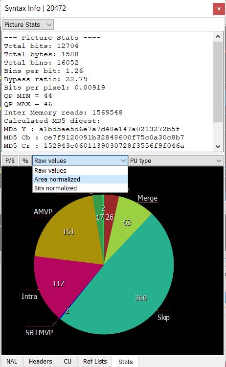
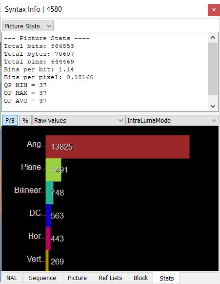
The bottom part displays pie/bar charts for several metrics depending on the type of statistics chosen in the top panel. The P/B button switches between Pie and horizontal Bar charts. Pressing % buttons changes the values in the corresponding view to the percentage view.
The first combo box in the panel of the bottom half allows to select between Raw values, Area normalized, Bits normalized to reflect different types of data to be represented in the statistics. Each pie/bar chart can be drawn normalized or un-normalized. Normalized data is weighted by area or compressed bits (Area normalized and Bits normalized options correspondingly). For example, there may be a much lower number of 64x64 CUs than 8x8 CUs in the picture (smaller un-normalized pie wedges), but they could still make up the majority of the picture area, making the 64x64 pie wedge large. Normalized numbers in the pie/bar chart are in units of pixels or bits, and un-normalized numbers are raw counts (Raw values option).
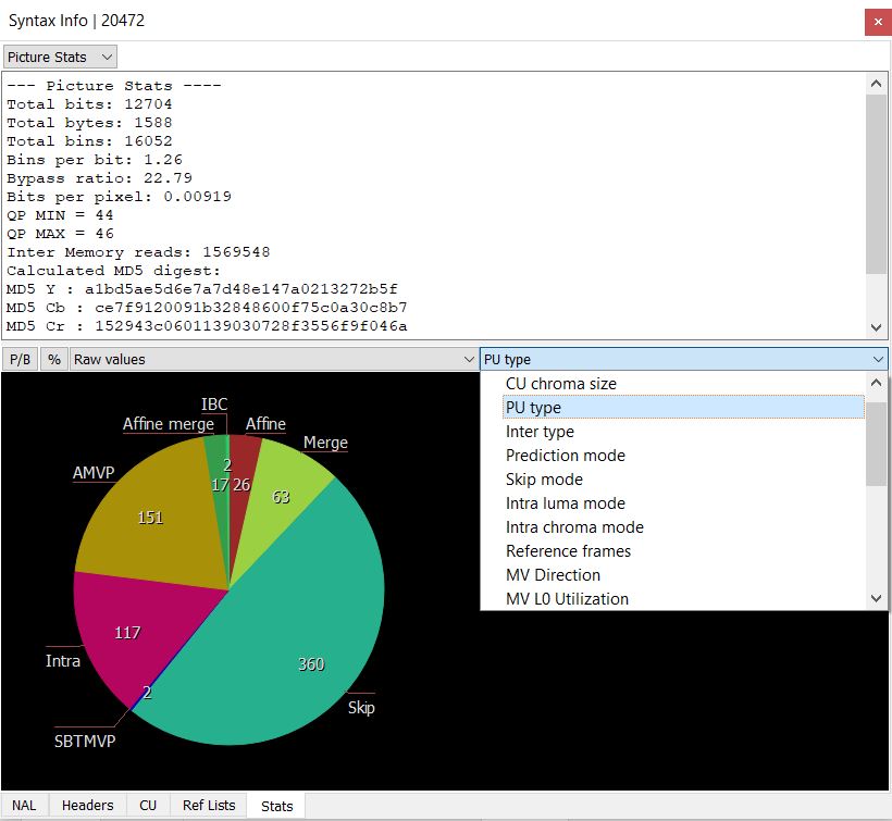
The second combo box allows to select between CU luma size, CU chroma size, PU type, Inter type, Prediction mode, Intra luma mode, Intra chroma mode, Intra chroma separated mode, Reference frames, MV Directions, MV L0 Utilization, MV L1 Utilization, TU luma size, TU chroma size, TU type Y, TU type U, YU type V, Non - zero coeffs Y, Non - zero coeffs U, Non - zero coeffs V, QP, Syntax element bin types, Memory reads for drawing statistics. Pie/bar charts for stream statistics show the accumulated values.
The pie/bar chart can be moved by dragging the mouse, and zoomed with the mouse scroll wheel.
Statistics information is also available in Info Overlays mode (when Info Overlays is selected in Mode in Main panel). For the description of this functionality see Overlays Info description in Modes.
Syntax Info panel can be switched on/off by ticking/unticking Syntax Info in View in Main menu. When switched on, it is displayed in the left side of the UI as a resizable panel with several tabs located at its bottom. The tabs display information about the syntax of the selected picture and the stream (see Stream View panel description). Bringing the mouse to the tab name shows explanation of its abbreviated name. The following subsections describe each tab in Syntax Info panel.
NAL (Network Abstraction Layer Units) tab displays a table with all units in the bitstream in decode order.
Above the list of the units the total number of units is displayed. The table has the following columns:
Pos - byte position of the unit in the file,
NAL Idx: Type: Name - NAL's index, start code value, start code type,
LId - Layer ID of the unit,
Tld/Value - Temporal ID of the unit/value of syntax element
Size - total number of bytes in the unit.
The unit descriptions are colored white or gray in blocks. Units in each block belong to one picture. Therefore, a change in color indicates a picture border.
In the second column, for some units there is a branch sign. Clicking on it, rolls out unit syntax elements as read from the bitstream. For each syntax element, VQ Analyzer shows its value and the number of bits it occupies in the bitstream. Red elements signal an error syntax element.
Clicking on any unit will display information on raw bytes of the unit in Unit Info panel. (For this, Unit Info panel needs to be switched on in View in Main panel.) Unit Info tab will show up to the first 500 raw bytes of the unit. Hex View Tab will highlight in yellow all raw bytes belonging to this unit.
Any unit can be double-clicked in order to bring forward the picture it belongs to as the current picture. Selecting a block in the Main panel will highlight the unit containing the patch with the selected block in NAL tab.
At the bottom of the unit tab is a button called Extract selected units. Clicking this button will write all the selected units out to a file.
At the bottom of the unit tab there also a combo box which allows to select or filter the units in the list. By default it is set to No Filter.
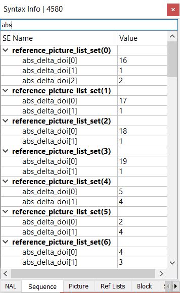
Sequence (Sequence Header) tab shows all syntax elements (SE) decoded in the sequence header and sequence extension header with values.
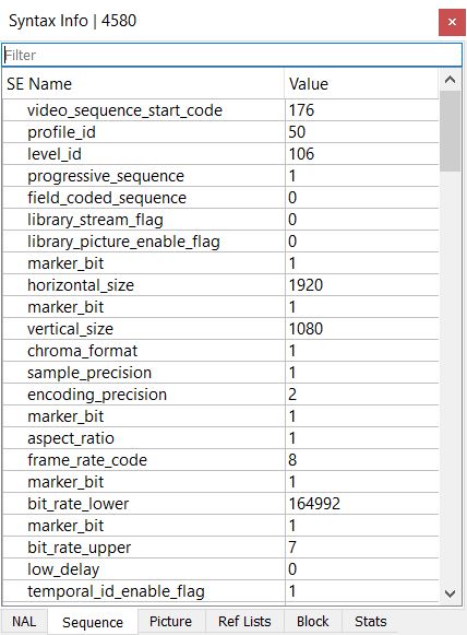
Right-clicking the mouse opens up a context menu with the following functionality:
Filter box allows to search for a SE by its name.
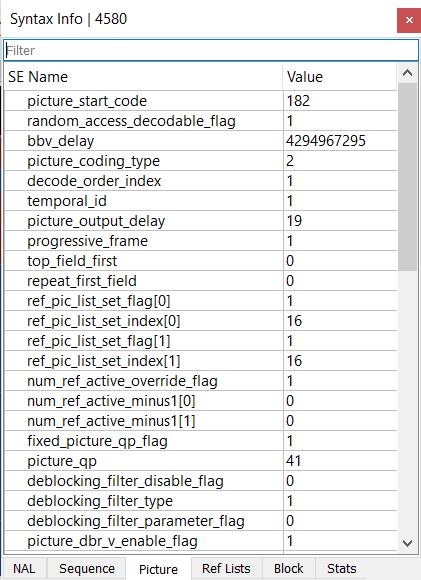
Picture (Picture Header) tab shows all syntax elements decoded in the picture header, picture coding extension, picture display extension and picture spatial scalable extension with values.
Right-clicking the mouse opens up a context menu with the following functionality:
Filter box allows to search for a SE by its name.
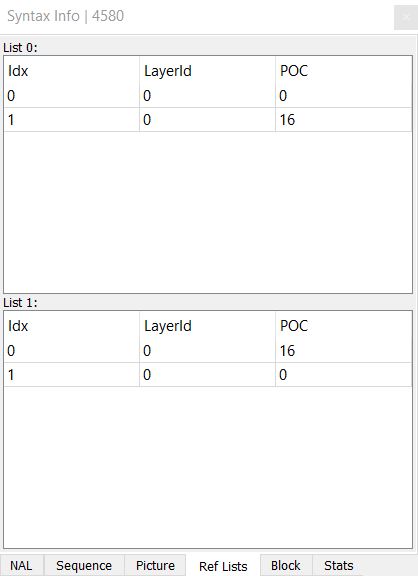
Ref Lists (Reference Lists) tab displays details of reference lists L0 and L1. L0 and L1 lists have the following columns:
Idx - Index associated with the reference picture Layer Id - Layer Index POC - Picture Order Count of the reference picture.
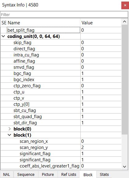
Block (Block-level syntax) tab displays the syntax elements (SE) associated with the currently selected block and their values. For this information to be displayed, a block needs to be highlighted by clicking the left button of the mouse in Main view.
Right-clicking the mouse opens up a context menu with the following functionality:
Filter box allows to search for a SE by its name.
Stats (Statistics) tab displays various types of statistics in the bitstream, namely picture statistics, per syntax element statistics, and overall stream statistics. This panel has two parts - top and bottom.
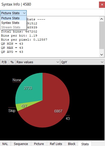
The top part gives an option of selecting between Picture Stats, Syntax Stats, and Stream Stats **in the combo box. **Picture Stats gives picture statistics, compression statistics as well as the image digest information. It also provides some min/max/average information about selected picture parameters, such as QP value, MVs. etc.
Syntax Stats lists Counts and Bits for each syntax element of the current picture. They can be displayed as numbers or % if you click % button which appears next to Syntax Stats button.
Stream Stats lists Counts and Bits for the syntax elements of the entire stream. Overall stream statistics is available only after after Run full stream analysis is performed by pressing the round blue button located on the top panel of Stream View. (Stream View panel needs to be opened in Main menu to do it.) Counts and Bits can be displayed as numbers or % if you click % button which appears next to Stream Stats button.
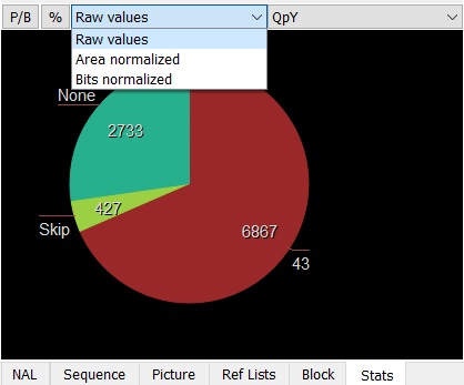
The bottom part displays pie/bar charts for several metrics depending on the type of statistics chosen in the top panel. The P/B button switches between Pie and horizontal Bar charts. Pressing % buttons changes the values in the corresponding view to the percentage view.
The first combo box in the panel of the bottom half allows to select between Raw values, Area normalized, Bits normalized to reflect different types of data to be represented in the statistics. Each pie/bar chart can be drawn normalized or un-normalized. Normalized data is weighted by area or compressed bits (Area normalized and Bits normalized options correspondingly). For example, there may be a much lower number of 64x64 CUs than 8x8 CUs in the picture (smaller un-normalized pie wedges), but they could still make up the majority of the picture area, making the 64x64 pie wedge large. Normalized numbers in the pie/bar chart are in units of pixels or bits, and un-normalized numbers are raw counts (Raw values option).
The second combo box allows to select between CU size, CU Mode, Intra Chroma Mode, Intra Luma Mode, QpY, and TU size for drawing statistics. Pie/bar charts for stream statistics show the accumulated values.
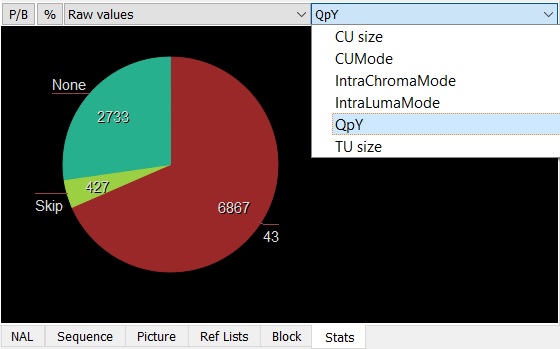
The pie/bar chart can be moved by dragging the mouse, and zoomed with the mouse scroll wheel.
Statistics information is also available in Info Overlays mode (when Info Overlays is selected in Mode in Main panel). For the description of this functionality see Overlays Info description in Modes.
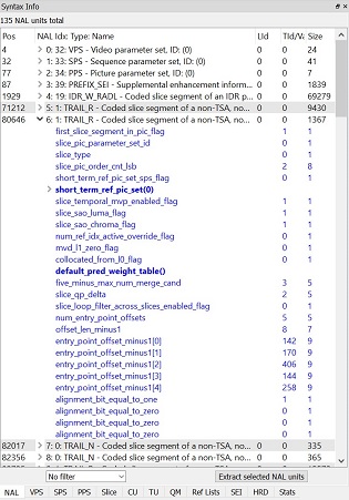
NAL tab lists all units found in the bitstream, in decode order. Above the list the total number of units is displayed. The list has five columns: "Pos" is the byte position of the unit in the file, "Unit Type" is the textual description of the unit's type, "LId" is the Layer ID of the unit, "TID" is the Temporal ID of the unit, and "Size" indicates the total number of bytes in the unit.
Changes in coloring from white to grayscale and back show the Access Unit borders. By clicking on the branch sign you can roll out unit syntax elements as read from the bitstream. For each syntax element, the VQ Analyzer shows the value of it and the number of bits it takes in the bitstream. Red elements will help you to identify error syntax element.
Clicking on any unit will display up to the first 500 raw bytes in the Unit Info panel. If a unit is a VCL unit, meaning it is a coded slice segment, it can be double-clicked in order to bring forward the picture it belongs as the current picture. Conversely, changing the current picture will highlight the unit that contains the first slice segment of that picture. Selecting a CU in the Main Panel will highlight the unit containing the slice that contains the selected CU.
At the bottom of the unit tab is a button called "Extract selected units". Clicking this will write all selected units out to a file.
These tabs contain a list of every syntax element, in decode order, of the VPS, SPS, Slice segment header and SEI messages that apply to the currently selected CU in the Main Panel. Syntax elements that come from a sub-function call are indented accordingly, and the function call itself appears in the list as a syntax element with no value. Any part of the list can be selected and copied for pasting in other programs.
This panel displays the syntax elements associated with the currently selected block.
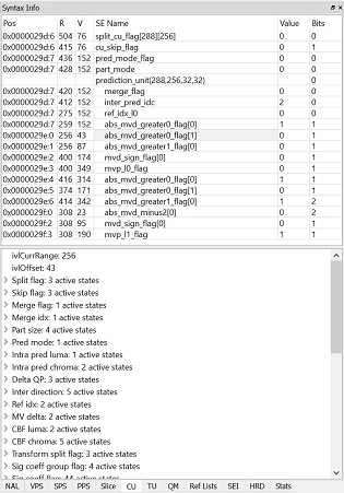
These tabs contain a list of the CABAC syntax elements decoded, in decode order, of the currently selected CU or TU in the Main Panel. Note that only the syntax elements pertaining to the currently selected CU/TU are shown, not any of the syntax elements in a higher or lower nodes in the quadtree. So if a CU is selected that is split into 4 smaller CUs, only the split flag will be shown, not the syntax elements of CUs further down the quadtree.
The left side of the list contains two columns, R and V, which denote the state of the CABAC engine's Range (ivlCurrRange) and Value (ivlOffset) prior to the syntax element decoding process. Any part of the list can be selected and copied for pasting in other programs.
Clicking a syntax element will update the tree in the lower half of this panel. This tree displays the values of all CABAC state variables prior to the decoding of the selected syntax element.
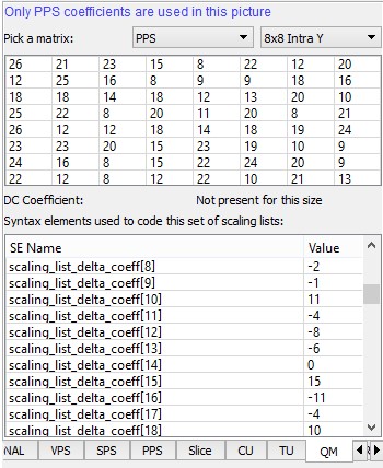
This tab displays the scaling lists, or quantizer matrices, used by the current picture. Scaling lists can be present in the SPS, PPS, or both. PPS scaling lists take precedence over SPS when present. The top of the panel shows in blue text how the various scaling lists are used in this picture. Below that, one of the 20 scaling lists from either the SPS or PPS can be chosen for inspection, and the chosen matrix is displayed in the grid. Matrices for 16x16 and larger TUs have a separate DC coefficient, which is displayed below the grid. Also shown in this panel is the list of syntax elements that is used to code the scaling list set, and is identical to the syntax in the corresponding SPS or PPS tab.
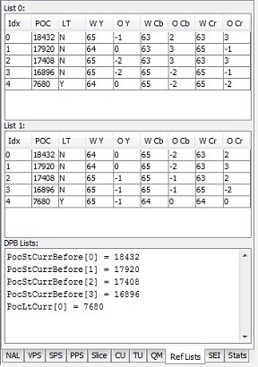
This tab displays the details of the two reference lists L0 and L1, as well as the Reference Picture Set arrays used to construct the L0 and L1 lists. The L0 and L1 lists have the following columns:
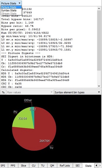
Stats tab displays various statistics extracted from the current picture. The top half shows some picture size and compression stats as well as the image digest information. There are also some min/max/average information about some picture parameters, such as QP value, MVs and so on, in this window.
The bottom half displays pie charts for a number of metrics. Each pie chart can be drawn normalized or un-normalized. Normalized data is weighted by area or compressed bits. For example, there may be a much lower number of 64x64 CUs than 8x8 CUs in the picture (smaller un-normalized pie wedges), but they could still make up the majority of the picture area, making the 64x64 pie wedge large. Normalized numbers in the pie chart are in units of pixels or bits, and un-normalized numbers are raw counts.
The pie chart can be moved by dragging the mouse, and zoomed with the mouse scroll wheel.
By selecting different modes in the stats combo box, you can explore different types of statistics in the bitstream, namely: picture statistics, per syntax element statistics, and overall stream statistics. Overall stream statistics is available only after a full stream analysis and shows accumulated values across the entire stream. Pie charts for stream statistics also show the accumulated values.
Pressing '%' buttons changes the values in the corresponding view to the percentage view. The P/B button switches between Pie and horizontal Bar charts.
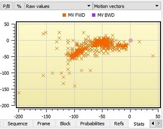
The inter-frame motion vector distribution can be viewed by selecting Motion vectors in the right combo box. This widget displays MV with maximum pel accuracy (1/4 pels) as 2D points. The user can switch separate MV values on or off by clicking on the corresponding MV legend.
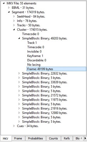
MKV tab represents the container type of the loaded stream.
VP9 streams using the WebM container will cause the UI to display the container's EBML document in tree form. Clicking an element causes the raw bytes coding that element to be displayed in the Raw Bytes panel (bottom center of the UI). When decoding a particular frame, the corresponding element will be highlighted in this panel. Other tracks may be present in the MKV file (such as audio), but they are not processed. The raw bytes can still be viewed though.
Frame tab shows all syntax elements decoded in the frame header, both the uncompressed and bool-coded partitions. A few stats about the size of the header are shown below the list.
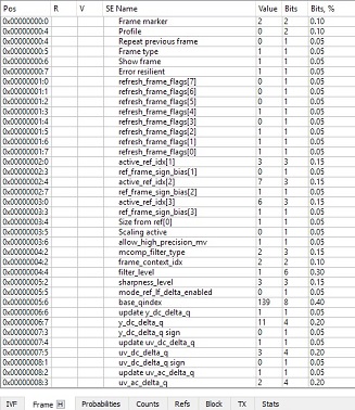
Since the VP9 reference software does not always assign a variable name to each decoded token, a descriptive name has been assigned which conveys the meaning or usage of the token.
The two left-hand columns R and V represent the value of the bool coder’s range and value prior to decoding the token. For the uncompressed part of the frame header, these values are not present.
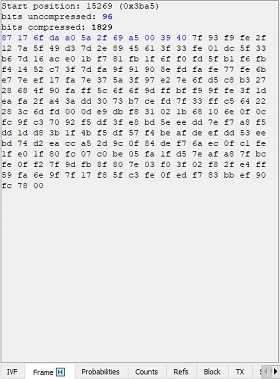
By pressing the ‘H’ button in the header tab you can see hexadecimal representation of the frame header. This representation shows all bytes of the header, starting position, and number of bytes in the compressed and uncompressed sections. Uncompressed bytes are highlighted in blue.
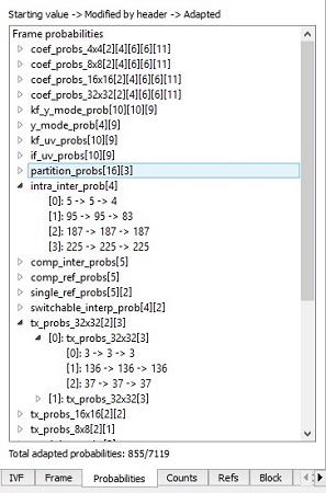
The probabilities used to decode the current frame are visible in this panel. They are organized hierarchically in the same way as the VP9 reference software. Each probability is given as three numbers. From left to right:
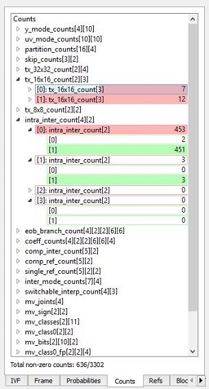
This tab shows the values of all the counters used for probability adaptation at the end of the frame decode. The counters are organized in hierarchical fashion in the same way as the VP9 reference decoder. Color bars give an indication of relative size of each counter in its group, and the parent icon contains the sum of the counts.
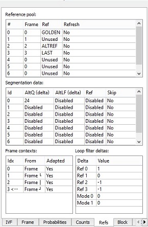
This panel displays the data that persists in the decoder between frames:
Since the VP9 reference software does not always assign a variable name to each decoded token, a descriptive name has been assigned which conveys the meaning or usage of the token.
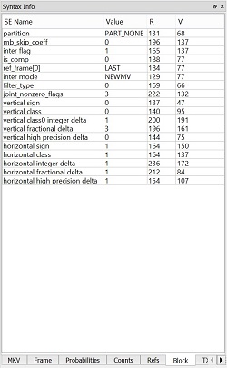
Note that only the syntax elements at the currently selected block hierarchy are shown. To see the PART_SPLIT tokens at higher levels in the recursive subdivision process, repeatedly click the same block in the main panel to navigate the hierarchy.
The two left columns R and V represent the value of the bool coder's range and value prior to decoding the token.
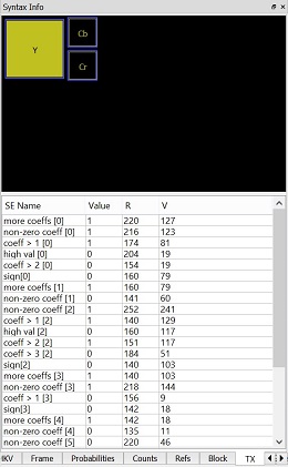
TX tab displays the syntax elements associated with the currently selected transform block. Since the VP9 reference software does not always assign a variable name to each decoded token, a descriptive name has been assigned which conveys the meaning or usage of the token.
A particular transform block may be selected in the Main Panel (when in Transform mode), or by clicking in the diagram above the syntax list. Note that when not in detail mode, only the luma transform blocks can be selected from the Main Panel.
The two left columns R and V represent the value of the bool coder's range and value prior to decoding the token.
Stats tab displays various statistics extracted from the current picture. The top half shows some picture size and compression stats as well as the image digest information. There are also some min/max/average information about some picture parameters, such as QP value, MVs and so on, in this window.
The bottom half displays pie charts for a number of metrics. Each pie chart can be drawn normalized or un-normalized. Normalized data is weighted by area or compressed bits. For example, there may be a much lower number of 64x64 CUs than 8x8 CUs in the picture (smaller un-normalized pie wedges), but they could still make up the majority of the picture area, making the 64x64 pie wedge large. Normalized numbers in the pie chart are in units of pixels or bits, and un-normalized numbers are raw counts.
The pie chart can be moved by dragging the mouse, and zoomed with the mouse scroll wheel.
By selecting different modes in the stats combo box, you can explore different types of statistics in the bitstream, namely: picture statistics, per syntax element statistics, and overall stream statistics. Overall stream statistics is available only after a full stream analysis and shows accumulated values across the entire stream. Pie charts for stream statistics also show the accumulated values.
Pressing the '%**' button changes the values in the corresponding view to the percentage view. The **P/B button switches between Pie and horizontal Bar charts.
The inter-frame motion vector distribution can be viewed by selecting Motion vectors in the right combo box. This widget displays MV with maximum pel accuracy (1/4 pels) as 2D points. The user can switch separate MV values on or off by clicking on the corresponding MV legend.
AV1 streams using Matroska container will cause the UI to display the container's EBML document in tree form. Clicking an element causes the raw bytes coding that element to be displayed in the Raw Bytes panel (bottom center of the UI). When decoding a particular frame, the corresponding element will be highlighted in this panel. Other tracks may be present in the MKV file (such as audio), but they are not processed. The raw bytes can still be viewed though.
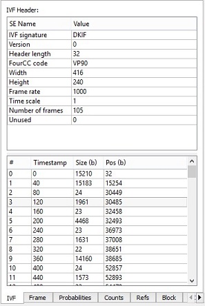
Streams containerized with the IVF format causes the UI to display the IVF information in this left-most tab. Selecting a frame makes the Raw Bytes panel show the raw bytes of that frame, including the IVF frame header. Clicking a frame will causes that frame to be decoded.
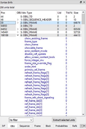
OBU tab lists all units found in the bitstream, in decode order. Above the list the total number of units is displayed. The list has five columns: "Pos" is the byte position of the unit in the file, "Unit Type" is the textual description of the unit's type, "LId" is the Layer ID of the unit, "TID" is the Temporal ID of the unit, and "Size" indicates the total number of bytes in the unit.
Changes in coloring from white to grayscale and back show the Access Unit borders. By clicking on the branch sign you can roll out unit syntax elements as read from the bitstream. For each syntax element, the VQ Analyzer shows the value of it and the number of bits it takes in the bitstream. Red elements will help you to identify error syntax element.
Clicking on any unit will display up to the first 500 raw bytes in the Unit Info panel. If a unit is a VCL unit, meaning it is a coded slice segment, it can be double-clicked in order to bring forward the picture it belongs as the current picture. Conversely, changing the current picture will highlight the unit that contains the first slice segment of that picture. Selecting a CU in the Main Panel will highlight the unit containing the slice that contains the selected CU.
At the bottom of the unit tab is a button called "Extract selected units". Clicking this will write all selected units out to a file.
For AV1 bitstream Sequence and Frame tabs are available.
Frame tab shows all syntax elements decoded in the frame header, both the uncompressed and bool-coded partitions. A few stats about the size of the header are shown below the list.
Since AV1 reference software does not always assign a variable name to each decoded token, a descriptive name has been assigned which conveys the meaning or usage of the token.
The two left-hand columns R and V represent the value of the bool coder’s range and value prior to decoding the token. For the uncompressed part of the frame header, these values are not present.
By pressing the ‘H’ button in the header tab you can see hexadecimal representation of the frame header. This representation shows all bytes of the header, starting position, and number of bytes in the compressed and uncompressed sections. Uncompressed bytes are highlighted in blue.
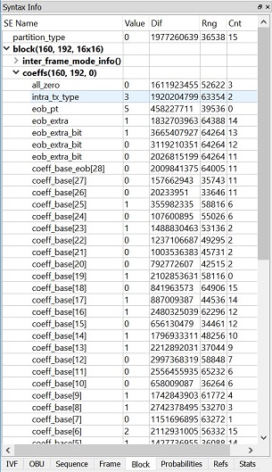
Since the AV1 reference software does not always assign a variable name to each decoded token, a descriptive name has been assigned which conveys the meaning or usage of the token.
Note that only the syntax elements at the currently selected block hierarchy are shown. To see the PART_SPLIT tokens at higher levels in the recursive subdivision process, repeatedly click the same block in the main panel to navigate the hierarchy.
The two columns Rng and Dif represent the value of the entropy coder's range and value prior to decoding the token. The Cnt column corresponds to the internal entropy coder counter.
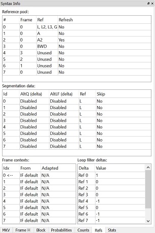
Refs tab displays the data that persists in the decoder between the frames:
This tab displays various statistics extracted from the current picture. The top half shows some picture size and compression stats as well as the image digest information. There are also some min/max/average information about some picture parameters, such as QP value, MVs and so on, in this window.
The bottom half displays pie charts for a number of metrics. Each pie chart can be drawn normalized or un-normalized. Normalized data is weighted by area or compressed bits. For example, there may be a much lower number of 64x64 CUs than 8x8 CUs in the picture (smaller un-normalized pie wedges), but they could still make up the majority of the picture area, making the 64x64 pie wedge large. Normalized numbers in the pie chart are in units of pixels or bits, and un-normalized numbers are raw counts.
The pie chart can be moved by dragging the mouse, and zoomed with the mouse scroll wheel.
By selecting different modes in the stats combo box, you can explore different types of statistics in the bitstream, namely: picture statistics, per syntax element statistics, and overall stream statistics. Overall stream statistics is available only after a full stream analysis and shows accumulated values across the entire stream. Pie charts for stream statistics also show the accumulated values.
Pressing '%' button changes the values in the corresponding view to the percentage view. The P/B button switches between Pie and horizontal Bar charts.
The inter-frame motion vector distribution can be viewed by selecting Motion vectors in the right combo box. This widget displays MV with maximum pel accuracy (1/4 pels) as 2D points. The user can switch separate MV values on or off by clicking on the corresponding MV legend.
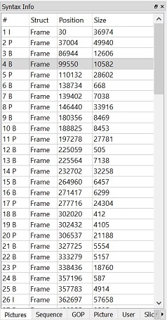
In Pictures tab, the VQ Analyzer presents the raw picture sequence with type, offset and size.
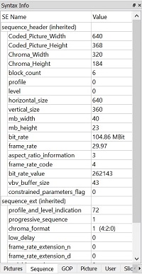
Sequence tab shows all syntax elements decoded in the sequence header and sequence extension header, both the uncompressed and bool-coded partitions.
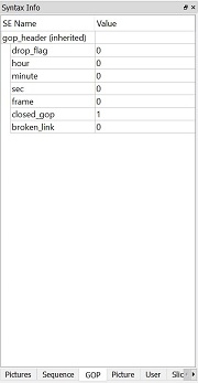
GOP tab shows all syntax element decoded in GOP header, both the uncompressed and bool-coded partitions.
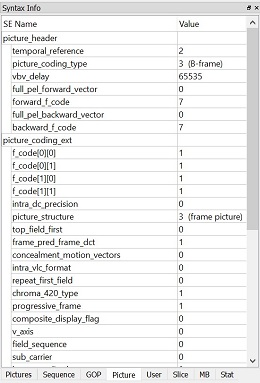
Picture tab shows all syntax element decoded in picture header, picture coding extension, picture display extension and picture spatial scalable extension, all of them are uncompressed and bool-coded.
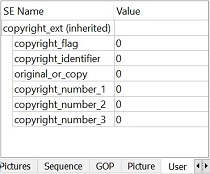
User tab displays the data that is decoded in user extension.
This tab displays various statistics extracted from the current picture. The top half shows some picture size and compression stats as well as the image digest information. There are also some min/max/average information about some picture parameters, such as QP value, MVs and so on, in this window.
The bottom half displays pie charts for a number of metrics. Each pie chart can be drawn normalized or un-normalized. Normalized data is weighted by area or compressed bits. For example, there may be a much lower number of 64x64 CUs than 8x8 CUs in the picture (smaller un-normalized pie wedges), but they could still make up the majority of the picture area, making the 64x64 pie wedge large. Normalized numbers in the pie chart are in units of pixels or bits, and un-normalized numbers are raw counts.
The pie chart can be moved by dragging the mouse, and zoomed with the mouse scroll wheel.
By selecting different modes in the stats combo box, you can explore different types of statistics in the bitstream, namely: picture statistics, per syntax element statistics, and overall stream statistics. Overall stream statistics is available only after a full stream analysis and shows accumulated values across the entire stream. Pie charts for stream statistics also show the accumulated values.
Pressing '%' buttons changes the values in the corresponding view to the percentage view. The P/B button switches between Pie and horizontal Bar charts.
The inter-frame motion vector distribution can be viewed by selecting Motion vectors in the right combo box. This widget displays MV with maximum pel accuracy (1/4 pels) as 2D points. The user can switch separate MV values on or off by clicking on the corresponding MV legend.
NAL tab lists all units found in the bitstream, in decode order. Above the list the total number of units is displayed. The list has five columns: "Pos" is the byte position of the unit in the file, "Unit Type" is the textual description of the unit's type, "LId" is the Layer ID of the unit, "TID" is the Temporal ID of the unit, and "Size" indicates the total number of bytes in the unit.
Changes in coloring from white to grayscale and back show the Access Unit borders. By clicking on the branch sign you can roll out unit syntax elements as read from the bitstream. For each syntax element, the VQ Analyzer shows the value of it and the number of bits it takes in the bitstream. Red elements will help you to identify error syntax element.
Clicking on any unit will display up to the first 500 raw bytes in the Unit Info panel. If a unit is a VCL unit, meaning it is a coded slice segment, it can be double-clicked in order to bring forward the picture it belongs as the current picture. Conversely, changing the current picture will highlight the unit that contains the first slice segment of that picture. Selecting a CU in the Main Panel will highlight the unit containing the slice that contains the selected CU.
At the bottom of the unit tab is a button called "Extract selected units". Clicking this will write all selected units out to a file.
These tabs contain a list of every syntax element, in decode order, of the SPS, PPS, Slice segment header and SEI messages that apply to the currently selected CU in the Main Panel. Syntax elements that come from a sub-function call are indented accordingly, and the function call itself appears in the list as a syntax element with no value. Any part of the list can be selected and copied for pasting in other programs.
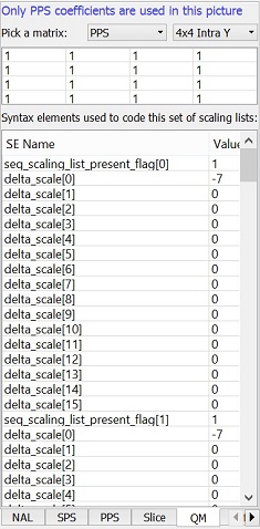
This tab displays the scaling lists, or quantizer matrices, used by the current picture. Scaling lists can be present in the SPS, PPS, or both. PPS scaling lists take precedence over SPS when present. The top of the panel shows in blue text how the various scaling lists are used in this picture. Below that, one of the 20 scaling lists from either the SPS or PPS can be chosen for inspection, and the chosen matrix is displayed in the grid. Also shown in this panel is the list of syntax elements that is used to code the scaling list set, and is identical to the syntax in the corresponding SPS or PPS tab.
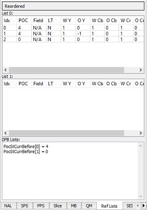
This tab displays the details of the two reference lists L0 and L1, as well as the Reference Picture Set arrays used to construct the L0 and L1 lists. The L0 and L1 lists have the following columns:
This tab displays various statistics extracted from the current picture. The top half shows some picture size and compression stats as well as the image digest information. There are also some min/max/average information about some picture parameters, such as QP value, MVs and so on, in this window.
The bottom half displays pie charts for a number of metrics. Each pie chart can be drawn normalized or un-normalized. Normalized data is weighted by area or compressed bits. For example, there may be a much lower number of 64x64 CUs than 8x8 CUs in the picture (smaller un-normalized pie wedges), but they could still make up the majority of the picture area, making the 64x64 pie wedge large. Normalized numbers in the pie chart are in units of pixels or bits, and un-normalized numbers are raw counts.
The pie chart can be moved by dragging the mouse, and zoomed with the mouse scroll wheel.
By selecting different modes in the stats combo box, you can explore different types of statistics in the bitstream, namely: picture statistics, per syntax element statistics, and overall stream statistics. Overall stream statistics is available only after a full stream analysis and shows accumulated values across the entire stream. Pie charts for stream statistics also show the accumulated values.
Pressing '%' buttons changes the values in the corresponding view to the percentage view. The P/B button switches between Pie and horizontal Bar charts.
The inter-frame motion vector distribution can be viewed by selecting Motion vectors in the right combo box. This widget displays MV with maximum pel accuracy (1/4 pels) as 2D points. The user can switch separate MV values on or off by clicking on the corresponding MV legend.
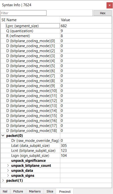
NAL tab displays a table with all units in the codestream in decode order.
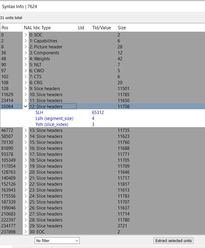
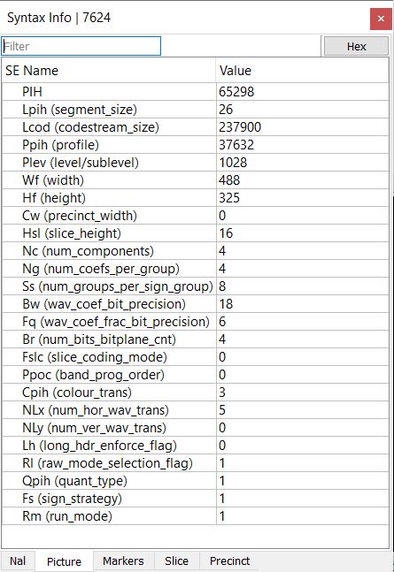
Picture tab shows all syntax elements decoded in the picture header.
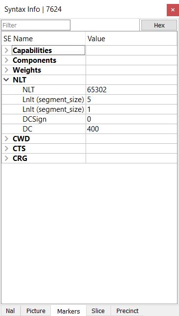
Markers tab shows all markers of the codestream and all syntax elements decoded in markers.
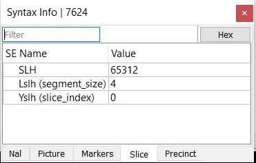
Slice tab shows all syntax elements decoded in the slice header with values for current slice.
Precinct tab shows all syntax elements decoded in the precinct header and packets for current precinct.
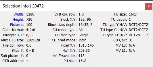
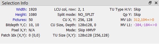
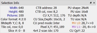
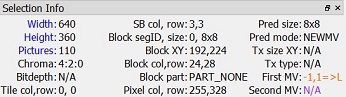
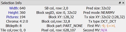
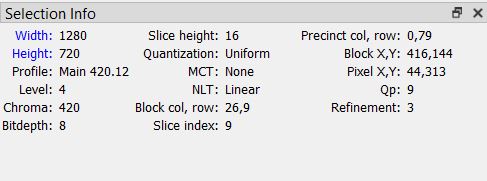
Selection Info panel is located at the bottom of UI. It provides details about the current selection at a glance.
All values are in decimal:
All values are in decimal:
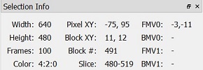
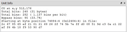
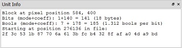
This panel shows a few details about the current selection at a glance:
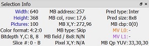
This panel shows a few details about the current selection at a glance:
This panel shows a few details about the current selection at a glance:
This panel shows a few details about the current selection at a glance. All values are in decimal:
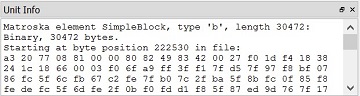
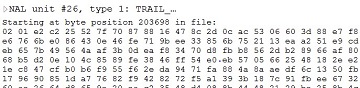
The panel in the bottom center of the UI displays the raw bytes that were used to code the selected block or NAL unit. The current selection can be a Matroska element/frame or an IVF frame (depending on the current bitstream’s container). A few details about the selection are included as well.
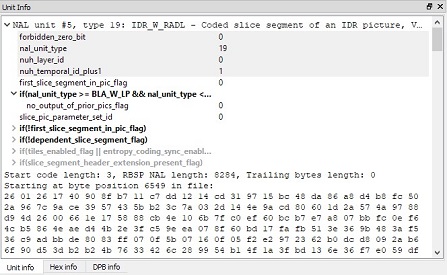
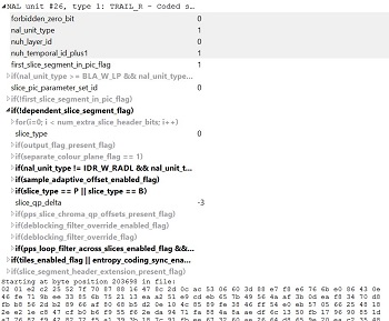
When you select an NAL unit in the NAL tab, the VQ Analyzer will immediately display up to the first 500 raw bytes in the Raw Bytes panel, and the controls for expanding NAL unit tree will appear from the left of the "NAL unit" keyword. Control representation is system-dependent.
By clicking on this control you can expand or collapse NAL unit tree items. The structure of this tree mostly replicates NAL unit definitions from the standard. There are items with statements and items with conditions. The items with conditions are greyed out if the condition is false. In this case, only the underlying structure definition from the standard is shown. Otherwise (if the condition is true), you can explore the real syntax values.
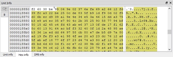
All supported codecs can be switched to Unit Info window in HEX View. This is implemented with a middle mouse double-click inside the Unit Info window. In this mode, the 'B' button switches between hex and binary representation. The yellow background highlights the currently selected Unit (e.g. NAL unit, CU, ...), showing start bit position on the first selected byte and end bit position on the last selected byte.
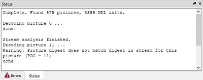
This tab in the lower left of the status panel displays messages about the decoding process and shows the progress of any actions that may take a while to complete. If a decoded picture's digest does not match the SEI digest (when present), a warning will be displayed here.
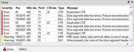
The errors tab at the bottom left of the panel turns red if the VQ Analyzer detects any errors/warnings in the stream. By clicking on this button, the VQ Analyzer switches to and from the list of detected problems. By double-clicking on the selected error, you can highlight the corresponding block in the main panel window, and the corresponding NAL unit will be highlighted.
The 3 numbers in the lower right of this panel represent the memory state of the process. From left to right the 3 numbers are:
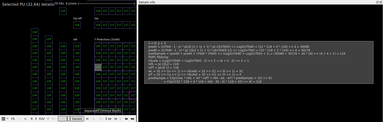
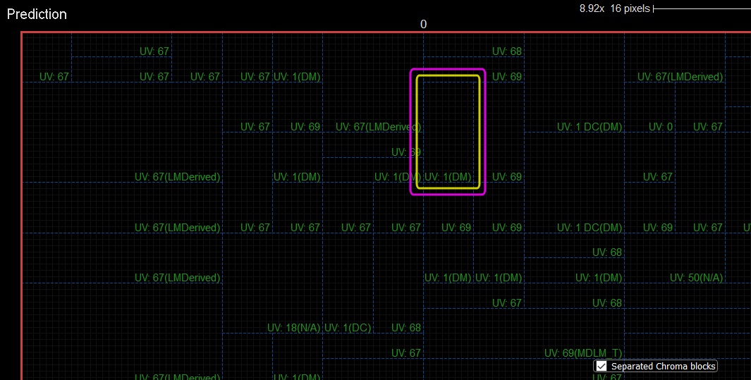
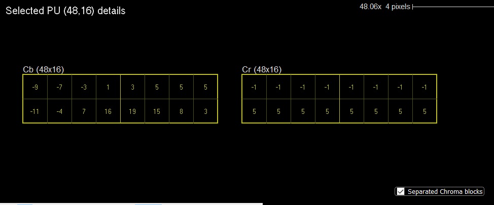
For VVC codec in the Prediction, Transform and Adaptive Filter modes, a popup with calculations for each pixel can be placed in a separate window Details info. This window can be turned on or off in the Options menu. The Details info window can be docked to the right or bottom of the main window, or it can be undocked by double-clicking the mouse and placed anywhere on the screen.
The following sections describe all specific features available when loading a VVC bitstream. The supported format of a bitstream is the raw bitstream with no surrounding container. Output from the publicly available VVC reference software HM is in this format and can be opened directly. VQ Analyzer supports Main, Main 10, and Main Still Picture profiles, VVC RExt profiles (including SCC), SHVC profile and VVC MultiView profiles. Sequences that go beyond the profile limits maybe be supported as well.
For I slices if separate coding tree syntax structure is used luma or chroma coding trees are displayed in main window. Use the check box in lower right corner for switching between luma and chroma.
In this case luma and chroma samples in detail mode will be presented separatly acording to check box.
Use Mode menu to see available modes.
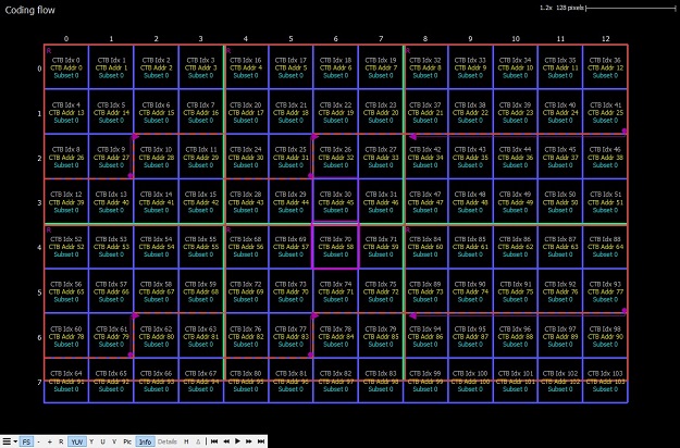
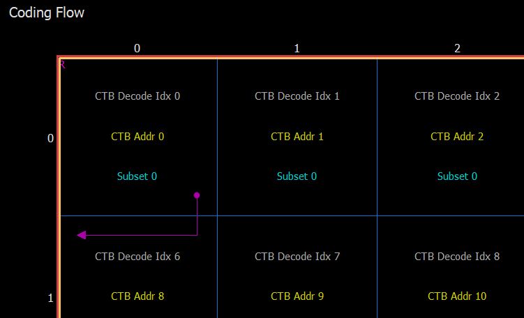
The coding flow mode gives a visual overview of CTBs. The blue grid shows the boundaries of the CTBs in the picture. Tile boundaries, when present, are shown with thick green lines, slice boundaries - with thick red lines and subpicture boundaries - with thick beige lines. Virtual boundaries are shown with thin light blue lines.
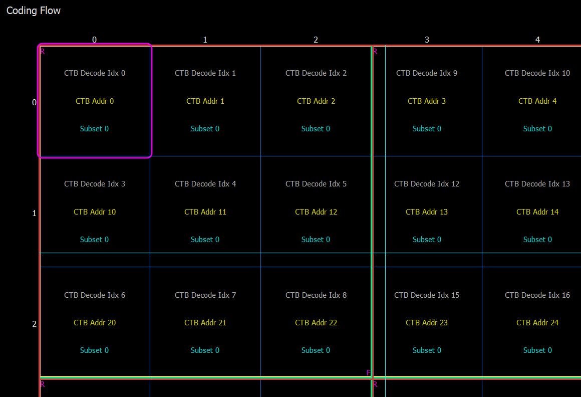
Each CTB contains 3 values:
The decode index of the CTB, showing the order of decode in the picture.
The CTB address, which is simply the raster scan index of the CTB.
The substream that the CTB belongs to. This number will only be greater than 0 if tiles or wavefront tools are employed in the picture.
Operations on the CABAC engine state are displayed as well. A small purple R at the top left of a CTB indicates the CABAC engine is reset before decoding that CTB. A small F indicates a CABAC flush at the end of a substream that is not the end of a slice. Purple arrows indicate CABAC engine state transfer or copy to dependent slices or wavefront rows.
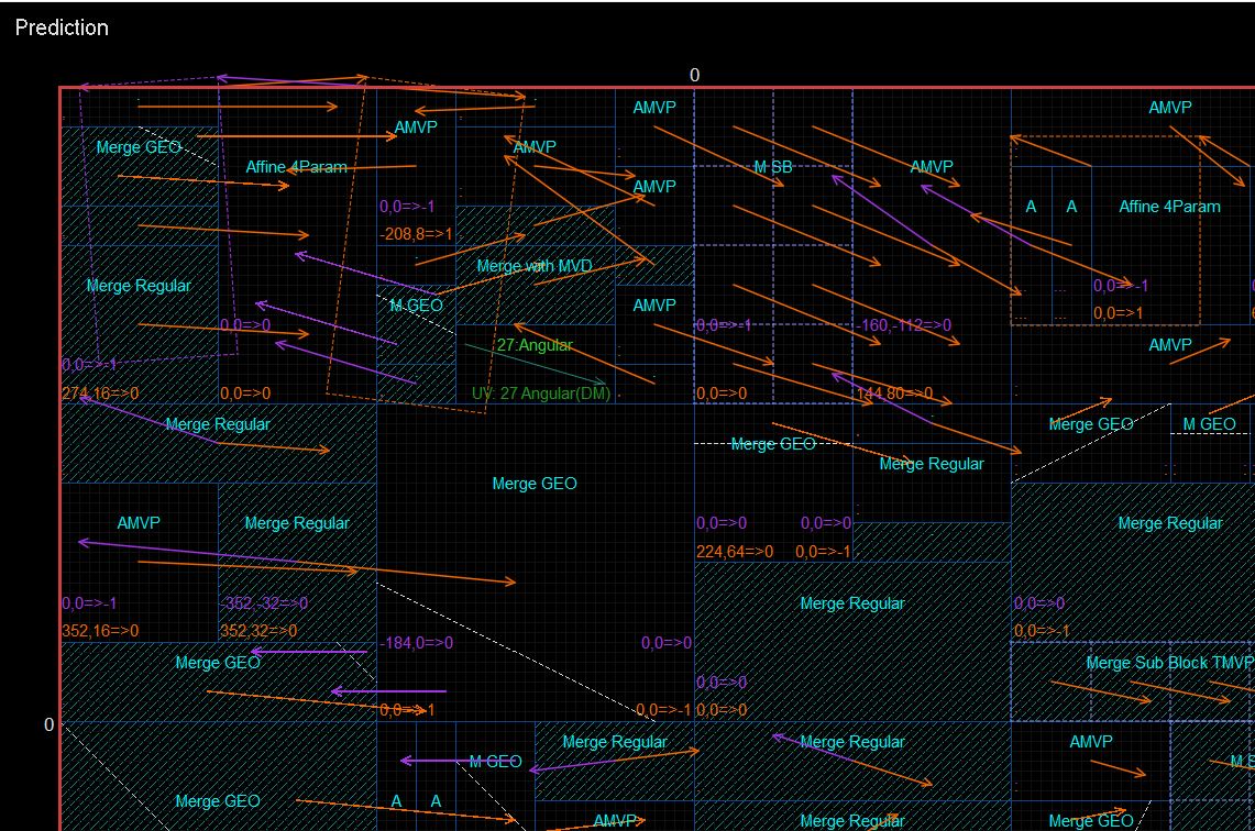
Intra modes are indicated with green colors, and directional modes also show an arrow indicating the prediction direction. In the lower right corner of an intra CU the chroma mode is indicated in a darker green.
Inter CUs are indicated with cyan colors showing the CU splits and mode. Additionally, skipped blocks are shaded with a lined texture. For AMVP, Merge Regular, Merge CIIP and MMVD inter CUs motion vectors are drawn in the block center. The L0 motion vectors are drawn in orange, the L1 motion vectors are drawn in purple. The MV value is shown in the lower left corner along with the reference index. For Merge GEO (GPM) inter blocks split line is drawn in dashed white, motion vectors are drawn in the center of each part and MV values are indicated on the bottom left for part A and on the bottom right for part B.
Clicking a CU will select it, and the syntax elements used to code it are displayed in the CU tab on the left. Clicking repeatedly on the same CU will cycle through the CU hierarchy, showing the parent and child relationship.
Below is shown Prediction mode on a zoomed-in selection along the top edge of a picture. The selected CU is surrounded with a pink box while the selected PU is surrounded with a yellow box.
For affine prediction blocks L0 and L1 motion vectors are drawn in the corners. Affine motion model is presented as dashed parallelograms.
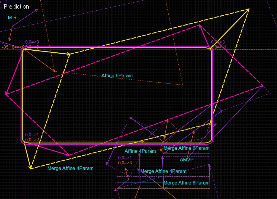
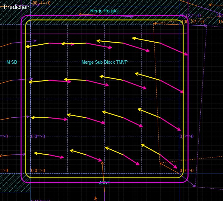
For Sub Block TMVP inter blocks motion vectors are drawn for each subblock of size 8*8. Sub Blocks borders are drawn in violet dashed lines.
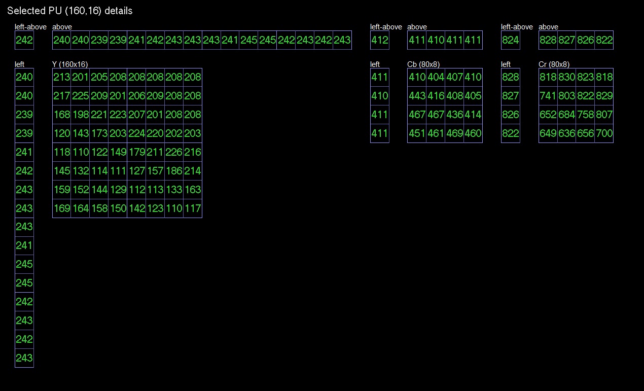
In prediction mode the sample values of a particular PU can be viewed in detail by right mouse click or "Details" button on main panel.
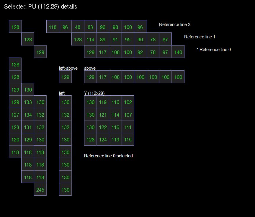
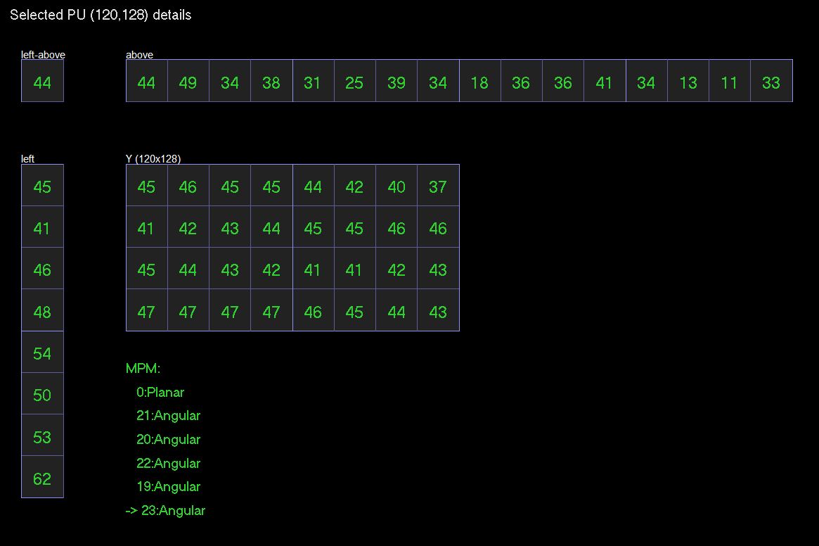
Intra PUs are displayed in green. The left, left-above and above prediction arrays are drawn next to the detailed samples.
If sps_mrl_enabled_flag is equal to 1 for intra blocks in details three reference lines of pixels (0, 1 and 3) is printed. The line selected for prediction is marked with an asterisk and label with this information.
If intra_luma_mpm_flag is equal to 1, a list of mode candidates is displayed for intra luma blocks in Details. The selected mode is marked with an arrow.
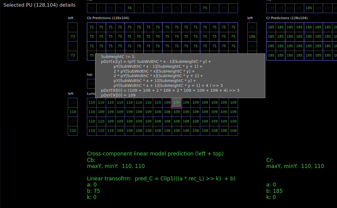
For the cross-component linear model modes (cclm_mode_flag = 1) additional info for chroma samples prediction is displayed in the Details. The reconstructed luma sample is displayed under the chroma component. The neighboring samples are displayed around chroma and down-sampled luma blocks. The selected neighboring samples are highlighted. Also, the linear model formula with parameters is displayed below. Each sample is clickable and the popup that appears shows the data for calculating it.
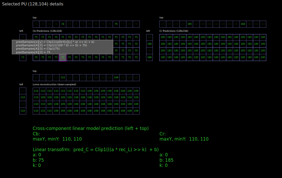
By clicking on each luma sample, a pop-up appears. Calculations of downsampling process is shown in popup.
For matrix-based intra prediction (mip_flag = 1) additional info for calculating prediction samples is available in Details. Reduced top and left boundary samples are displayed to the left and top of prediction samples.
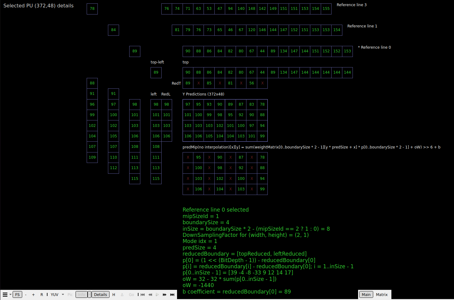
Matrix-based intra prediction samples are printed under prediction samples. Each sample is clickable and the popup that appears shows the data for calculating it.
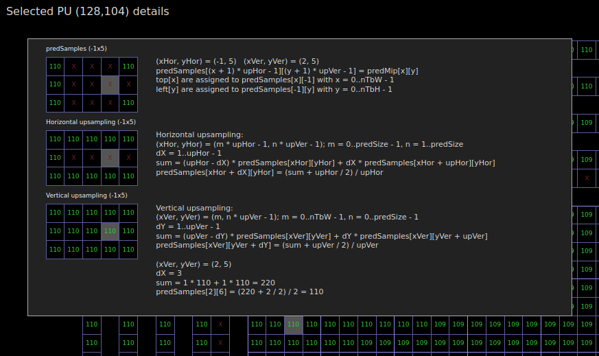
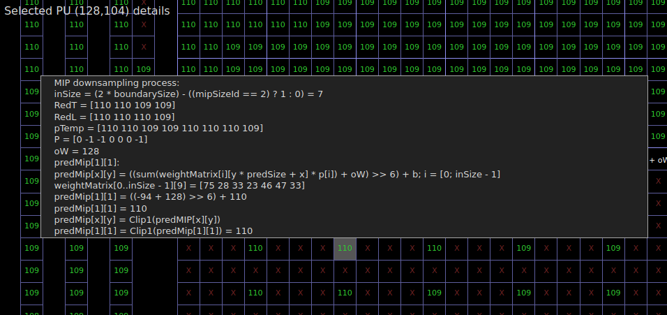
Parameters for calculating MIP samples are displayed below. Weights matrix can be expected in additional detailsby click on “Matrix info details”.
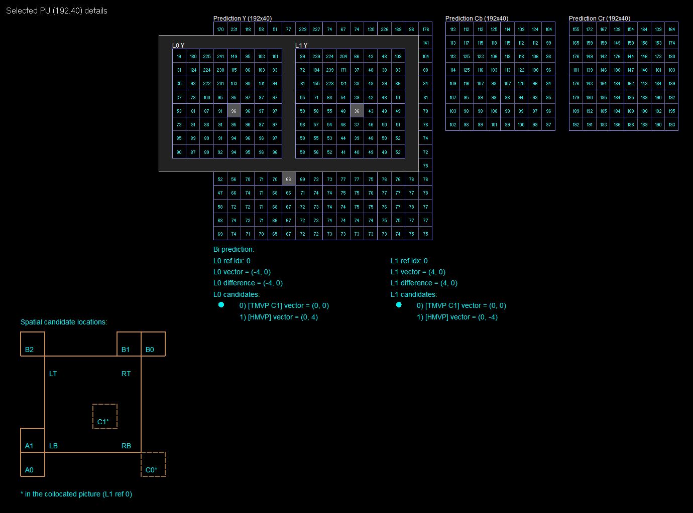
Inter PUs are displayed in cyan (turquoise).
For inter blocks the following information is displayed:
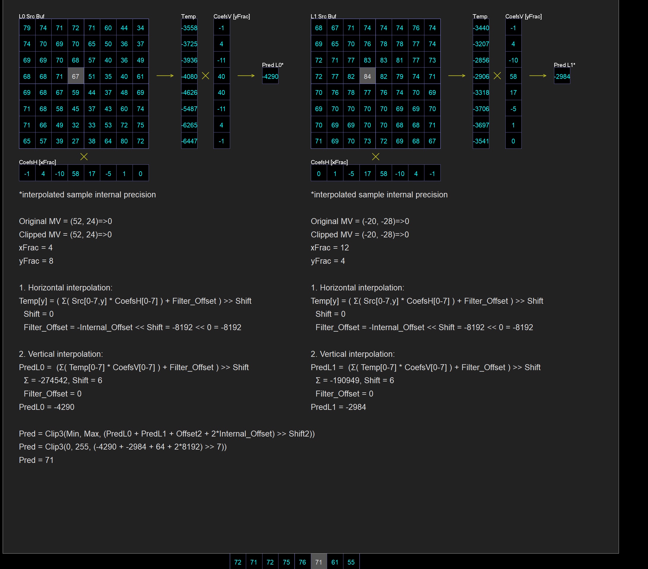
Additional prediction info is presented below:
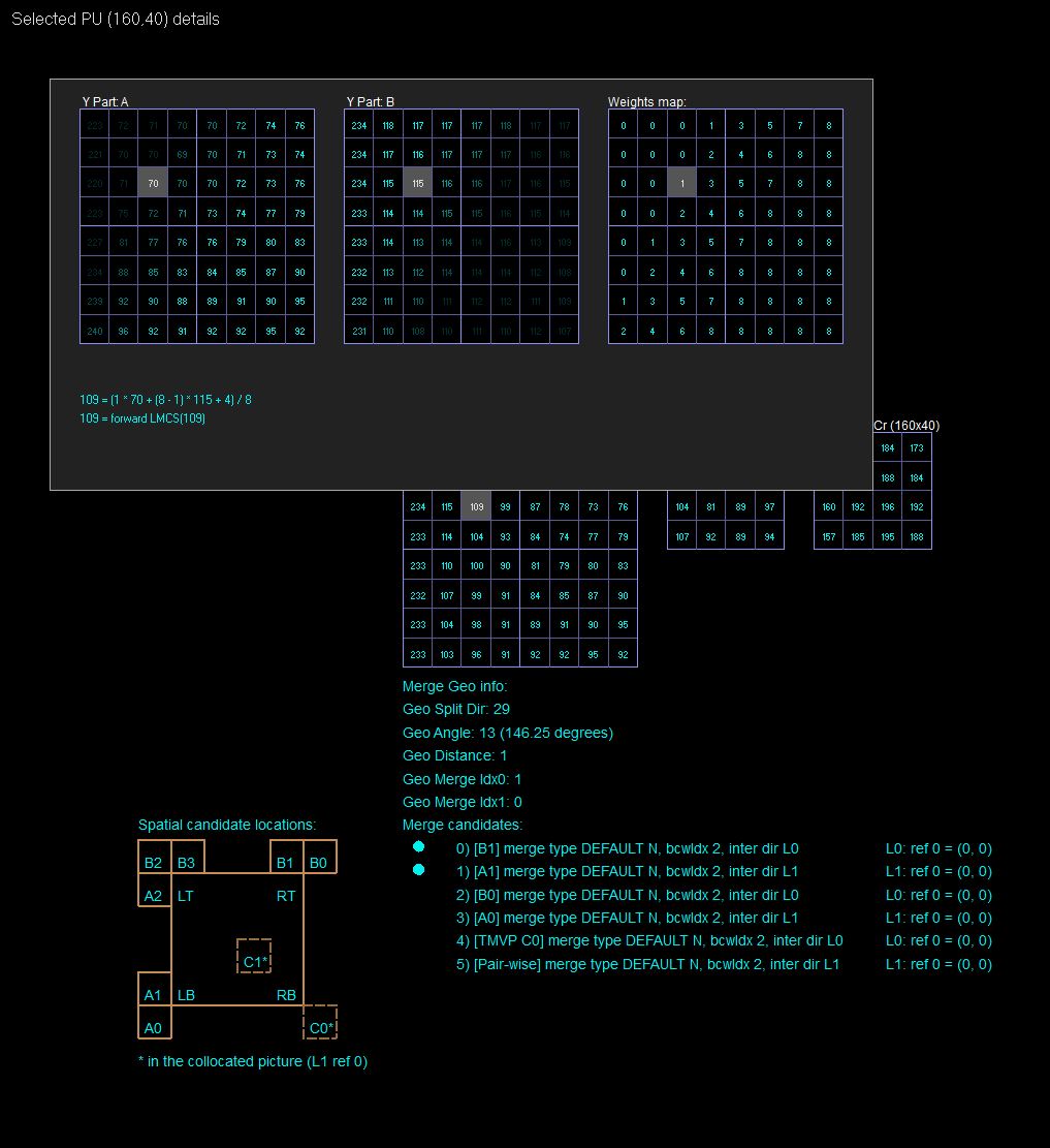
For GEO Merge blocks, split direction, angle, distance and two merge indices are indicated. Reference samples from part A and B, Weights map and the formula for calculating the current value of the pixel are shown in a popup window by clicking on the pixel. The brightness of the pixels in Part A and Part B depends on the coefficient of inclusion in the final block according to the Weights map. Pixels that fall into the final prediction (weights 8 and 0) are highlighted brightly. Pixels that are interpolated are highlighted paler (weights 1-7). Other pixels are darkened.
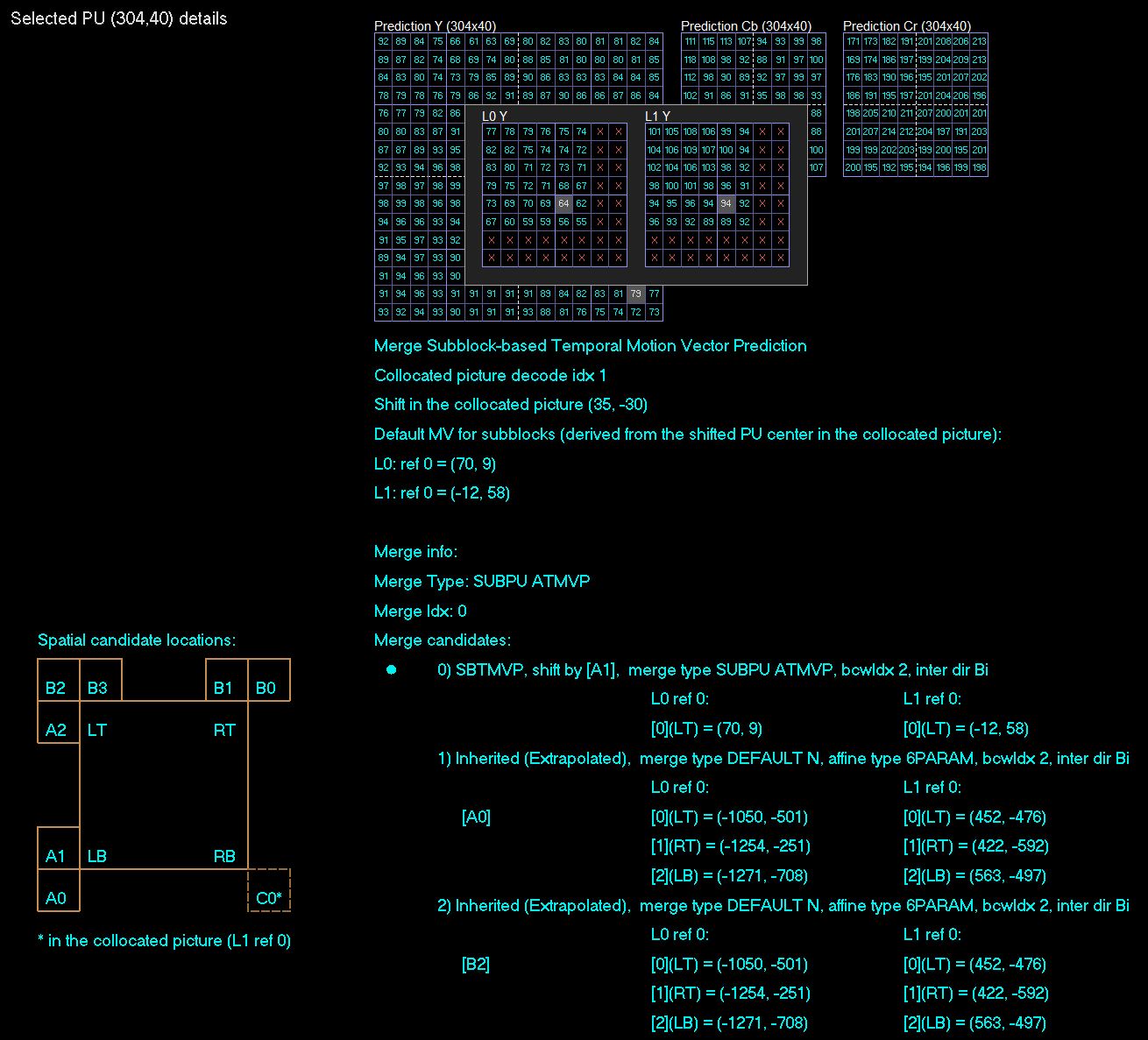
For Sub Block TMVP inter blocks collocated picture decode index, shift from collocated picture and default central motion vector are indicated. Sub block borders are drawn in white dashed lines.
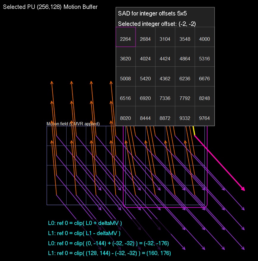
Motion Buffer mode is available for inter and IBC blocks in Details. In this mode motion vectors for each 4*4 blocks are displayed.
The values of the vector are printed below on mouse hover. If DMVR is applied in addition, the table 5*5 of SAD values is drawn in popup. Selected value has a pink border. Also in popup selected offset is printed. The motion vectors refinement calculation is printed at the bottom.
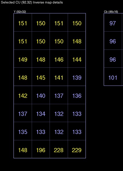
In Transform mode, transform trees and the accompanying residual signal of the picture are displayed.
As in Prediction mode, the boundaries of each CU are shown with thin blue lines. Transform splits (TUs), if present, are indicated with thin yellow lines. Within each CU/TU the following information on this CU/TU is provided: QP values (in the bottom left corner), the number of coefficients (in the top left corner), transform types (in the center). BDPCM-coded CUs are marked with "PCM" in white. ISP-coded CUs are marked with "ISP" in the bottom right corner. Intra Subpartition splits are indicated with dark green lines.
If the "Pic" button is turned on, the raw residual signal is shown in the image form. Transform values of 0 result in flat grey, negative values are darker and positive values are brighter.
Clicking a block, selects a TU with a light blue surrounding box and a CU with a purple one. A CU will be surrounded with a light blue and purple boxes if a TU coincides with a CU. Clicking a TU/CU repeatedly causes the selection to move up and cycle through the TU, then CU quadtree hierarchy.
To view full details of a particular TU, select the TU and enter Detail mode by either right clicking the mouse or using the detail view button (Details) at the bottom of the Main panel. The selected TU structure is arranged from top to bottom showing 3 major steps in recovering the residual signal:
If low frequency non-separable transformation (LFNST) process is applied, scaled transform coefficients after LFNST process (LFNST Coeffs) are additionally displayed after the transform coefficients. LFNST ID is then indicated next to the yellow arrow between the Transform Coeffs and LFNST Coeffs.
Clicking on the transform coefficient brings up a popup window with formulas and parameters for its calculation, excluding zero coefficients for dependent quantization (sh_dep_quant_used_flag = 1 ).
If joint coding of chroma residuals (JCCR) for chroma is applied, one transform coefficients and two residual samples blocks are shown with the indication of JCCR mode and sign flag.
Loop Filter mode shows all edges processed by deblocking filter. The edges are color coded in the following manner:
Green: Large filter applied Yellow: Strong filter applied Orange: Weak filter applied Red: No filter applied (but the edge was evaluated)
Additionally, colors of dashed lines classify edges by a block type:
Olive: coding unit (CU) edge purple: transform unit (TU) edge Teal: sub prediction unit (SubPU) edge Light blue: edges of SubPU and TU coincide
Clicking the L button in the upper right corner will open the legend explaining the color coding of the edges.
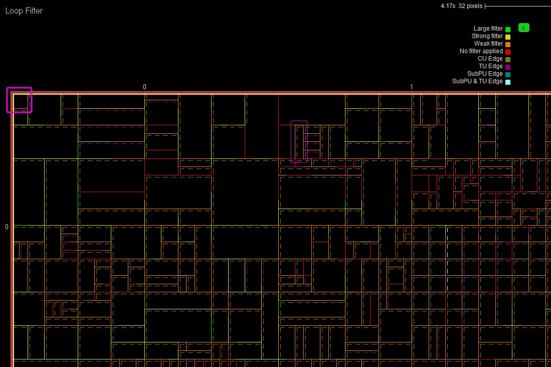
The deblocked sample values can be inspected in Detail mode. Sample values are colored yellow if they have been modified by the deblocking process. Filtered edges belonging to the selected CU are shown in thick dashed lines, color coded the same way as in the non-detail mode. Each edge can be selected and clicked upon, which will bring up a window with the input values to the edge filter. Additionally, the filter application options is displayed. Edges that were processed but ultimately not filtered are red colored. They can also be clicked on to view the parameters of the filtering process.
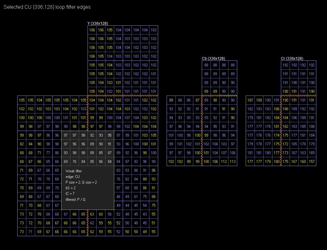
Clicking on a modified pixel will open up a window with the formula for calculating its value.
In SAO mode the SAO filter parameters are shown. The mode, and the associated four offsets for each component, are indicated with yellow text, and the merge_up / merge_left flags are indicated with an arrow.
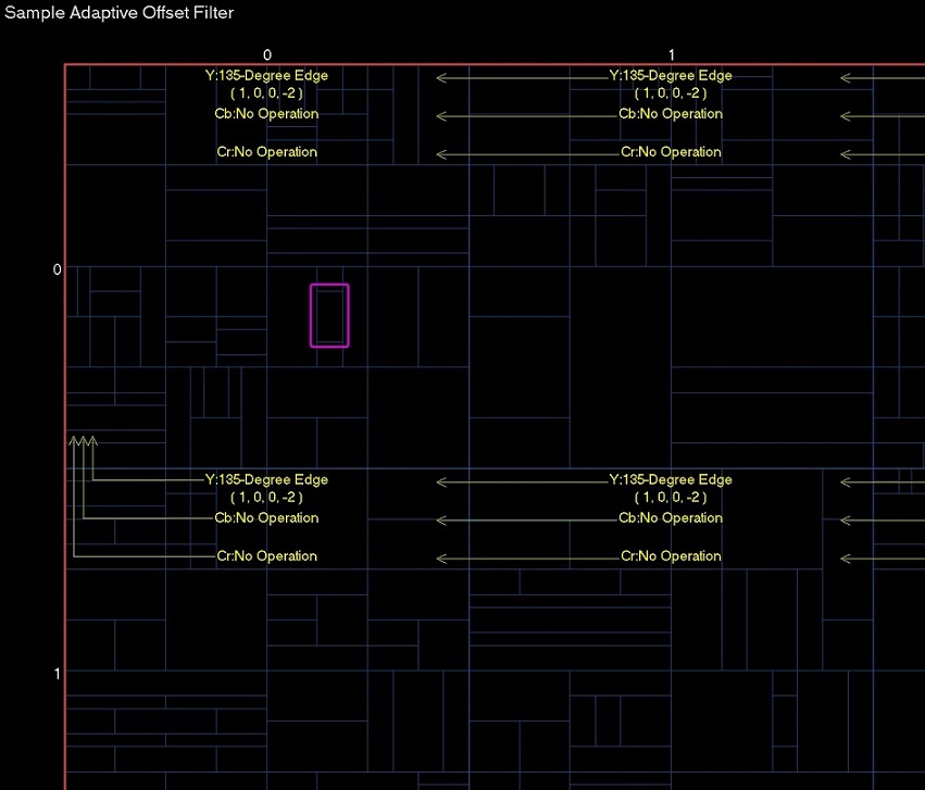
For SAO edge type, a 3x3 window with the input values to the filtering process and the formula for calculating output value appears. SAO edge offset class and specific offset values used in the filtering process are displayed below.
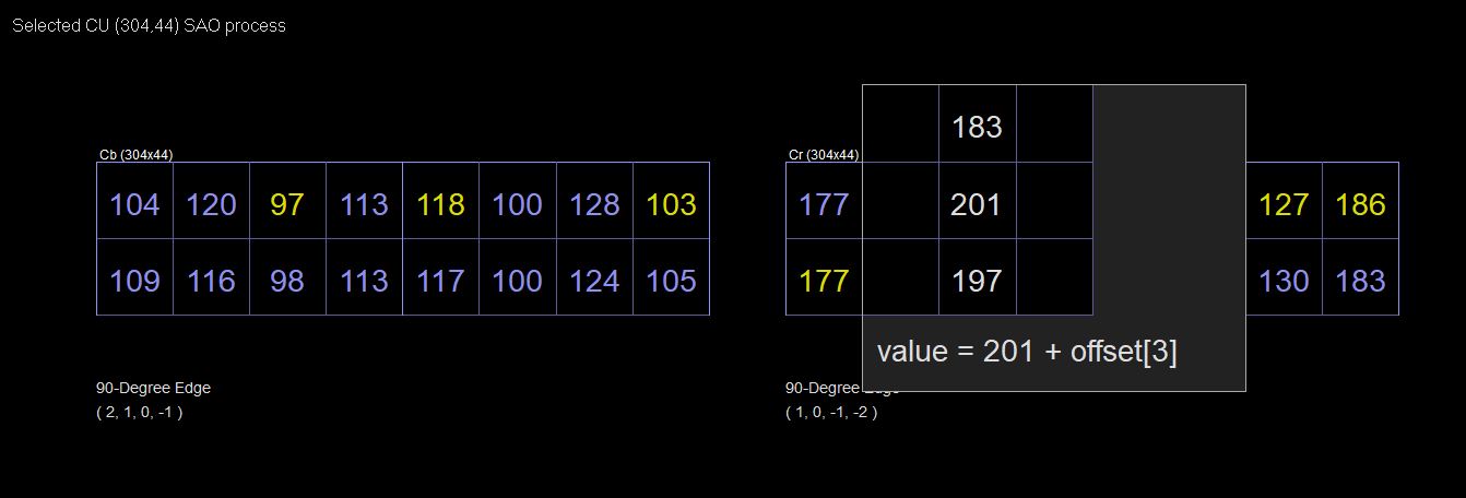
For SAO band type, a formula for calculating the value appears in a popup window by clicking on the pixel. The band position value and offset values in brackets are shown below.
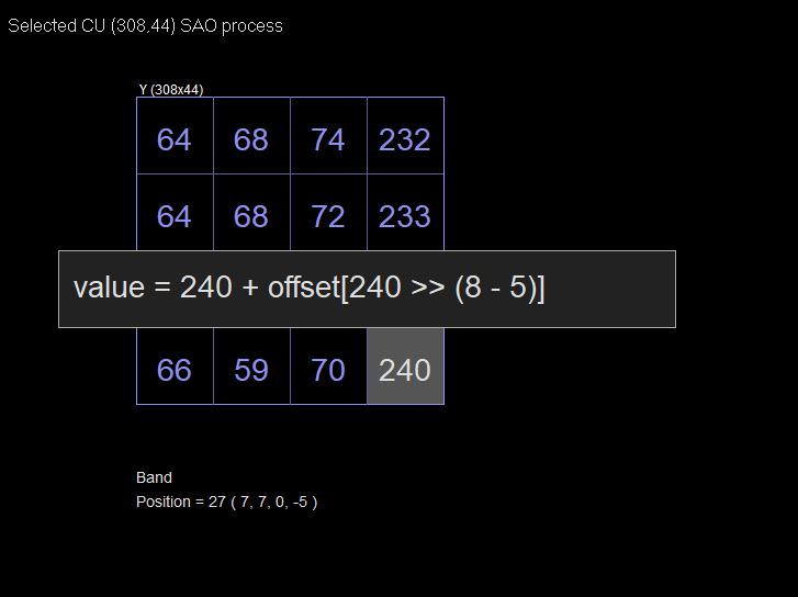
In Adaptive Filter mode, for each CTB, if available, the parameters of the adaptive loop filter are shown. The filter type and filter index for each component are indicated in yellow text. If the adaptive loop filter is not applied, "No operation" is written in yellow for this component.
For each 4*4 pixel block, the number before the dash and its color indicate the classification filter index. The arrow and the number after the dash indicate the transpose index. In the upper right corner, clicking on the L button brings up the legend with the explanation of the color coding of the indices. The "+" and "-" buttons near the depth label allow you to change the minimal selectable size of a picked block.
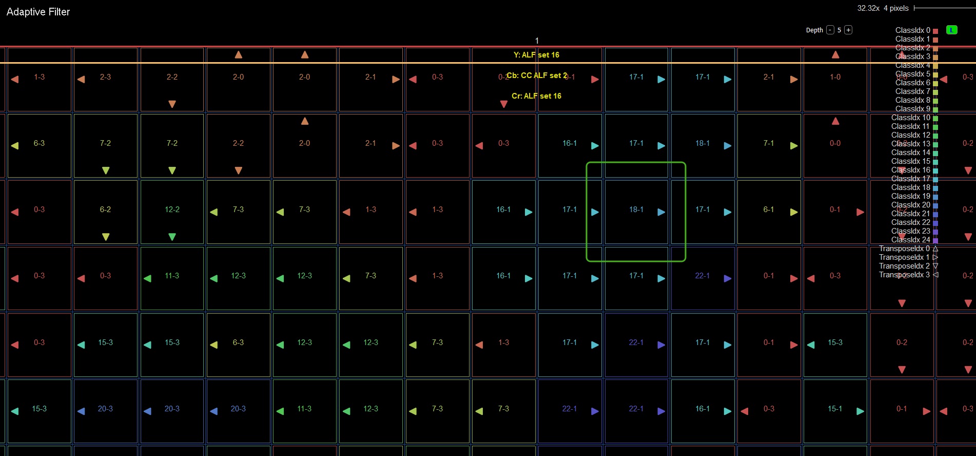
In Detail mode on a selected Block all samples processed by ALF filter are shown. Sample values that were modified by the ALF process are highlighted in yellow. Each sample can be clicked on. It will open a popup window with tables with parameters and formulas of ALF process, ALF coefficients, clipping values, and samples prior to ALF process. For chroma samples, if cross-component adaptive loop filter (CCALF) is applied, CCALF coefficients and corresponding luma samples (prior to ALF process) are shown in the popup window.
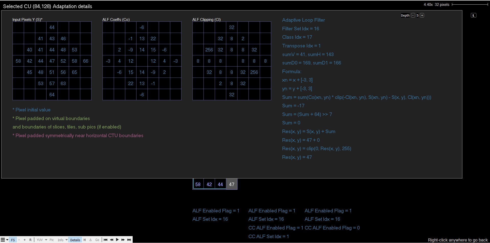
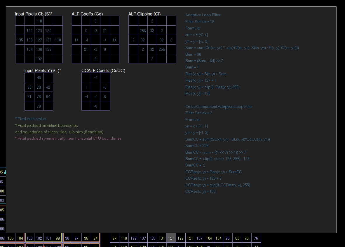
YUV mode allows the user to inspect the final decoded sample values, without additional overlay data.
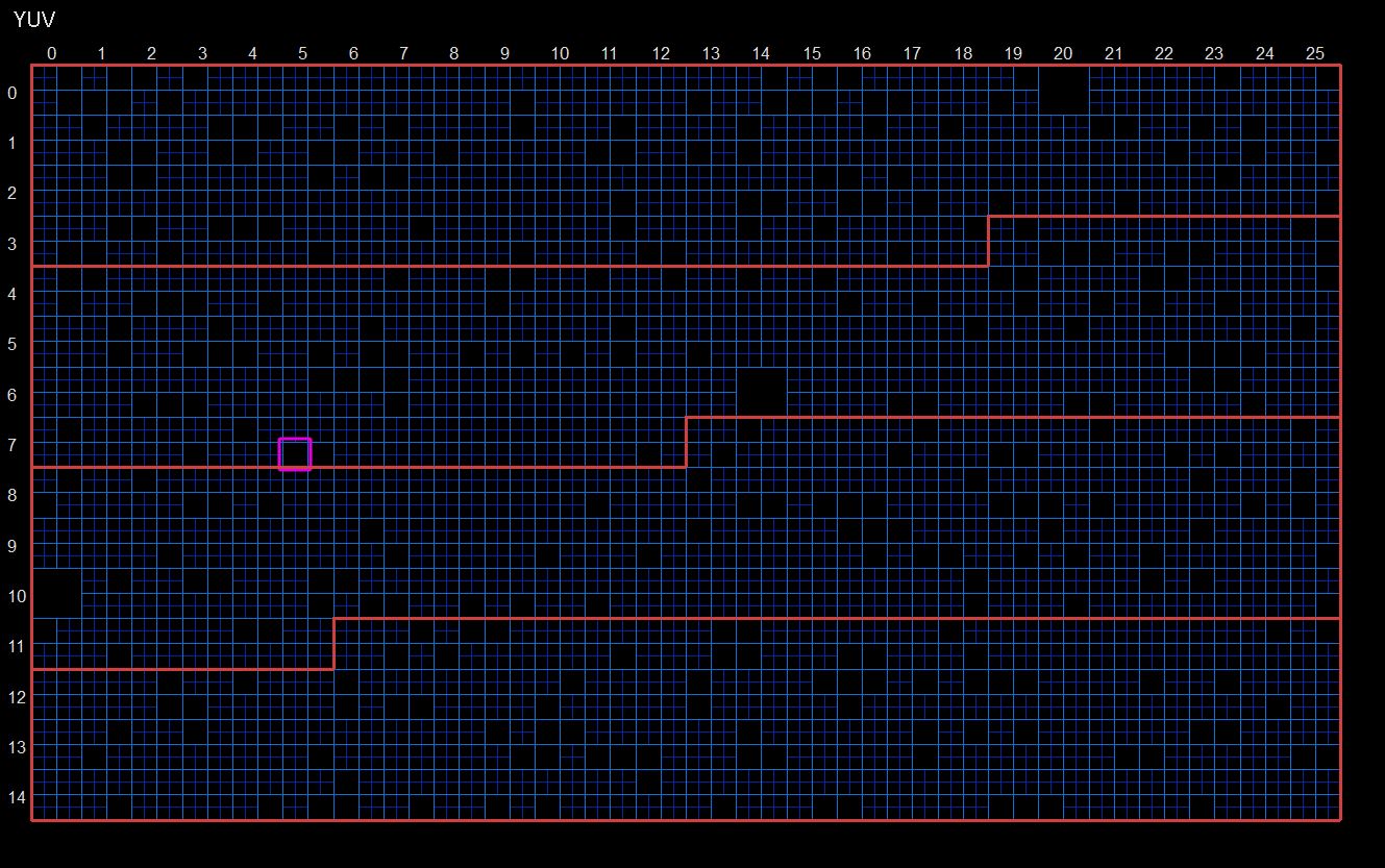
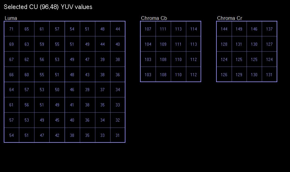
Overlays provide additional information about the picture that you're currently investigating. When you switch to "Info Overlays" mode, several additional submenus will appear in the bottom-left panel of info window.

You can switch now between additional modes with the drop down menu on the right. PSNR and SSIM modes are enabled if you have loaded a reference YUV file.
TBD
TBD
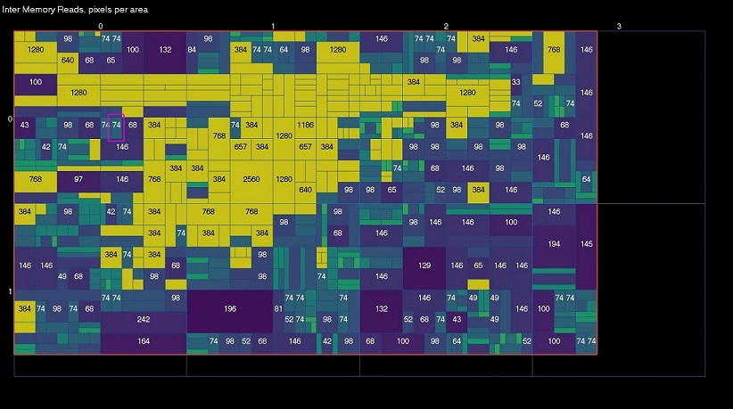
TBD
Prediction mode shows the PUs in each CU. Largest coding unit splits are indicated with blue lines.
When a CU split is implied by AVS3 and not directly coded in the bitstream, the split lines are dashed.
Intra modes are indicated with green colors. Directional modes like angular and SAWP (Spatial Angular Weighted Prediction) also show an arrow indicating the prediction direction. In the lower right corner of an intra PU the chroma mode is indicated in a darker green.
When the prediction shape is not the same as the CU size, the prediction unit shapes are shown with green lines for intra blocks (sub-prediction blocks) and cyan for inter blocks. Dashed green lines in intra blocks mean that the PU was split along with the transform tree.
Intra PUs have additional dark-green labels for IPF (Intra Prediction Filtering) and IIP (Improved Intra Prediction) modes used.
Intra Block Copy (IBC) and Intra String Copy (ISC) modes are indicated with cyan labels, also IBC has a block vector drawn in the center.
Inter PUs are indicated with cyan mode labels. The label indicates CU sub type, it is a combination of Skip, Inter, Direct types and Affine, AWP, UMVE, Etmvp and SbTemporal, Temporal, Spatial, MVAP, HMVP modes. The L0 motion vectors are drawn with an orange color, the L1 motion vectors (B slices only) are drawn with a purple color. The MV value is shown in the lower left corner along with the reference index.
Inter PUs have additional dark-cyan labels for showing filtering (BGC, IPF, IPC), refinement (DMVR, ASR) and prediction sample combination (BIO, OBMC, AWP).
Clicking a PU will select it, and the syntax elements used to code it and the CU it belongs to are displayed in the Syntax Info panel Block tab on the left-hand side (Syntax Info panel needs to be switched on in Main menu for this).
Clicking repeatedly on the same PU will cycle through the CU hierarchy, showing the parent and child relationship.
Below is shown Prediction mode on a zoomed-in selection along the top edge of a picture. The selected CU is surrounded with a pink box while the selected PU is surrounded with a yellow box.
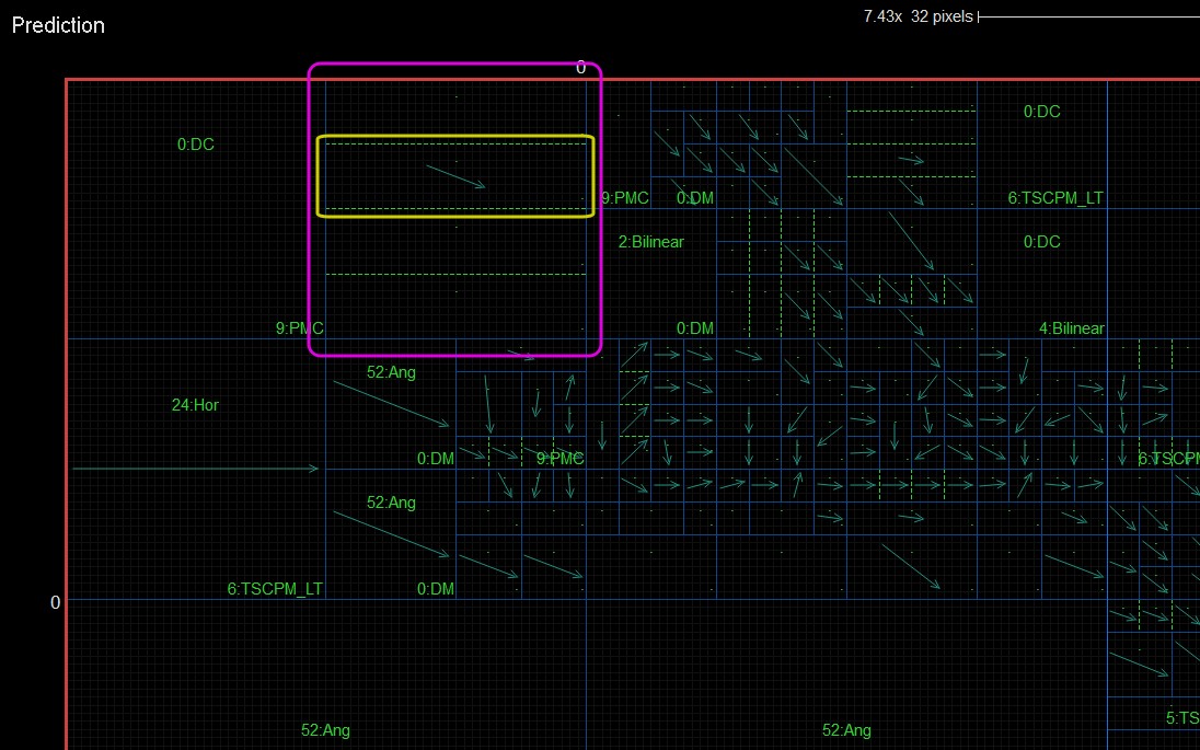
In Prediction mode, sample values of a particular PU can be viewed in Details.
Inter modes details show AMVR index, reference index, motion vector and difference.
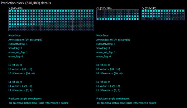
Also, additional special information for particular modes is displayed.
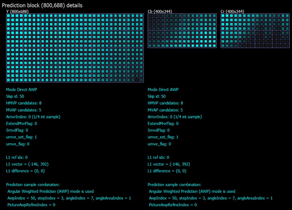
Intra String Copy (ISC) mode displays Ordinary and Non-ordinary mode details. For each mode strings with the parameters start pixels, lengths, types and vectors are displayed.
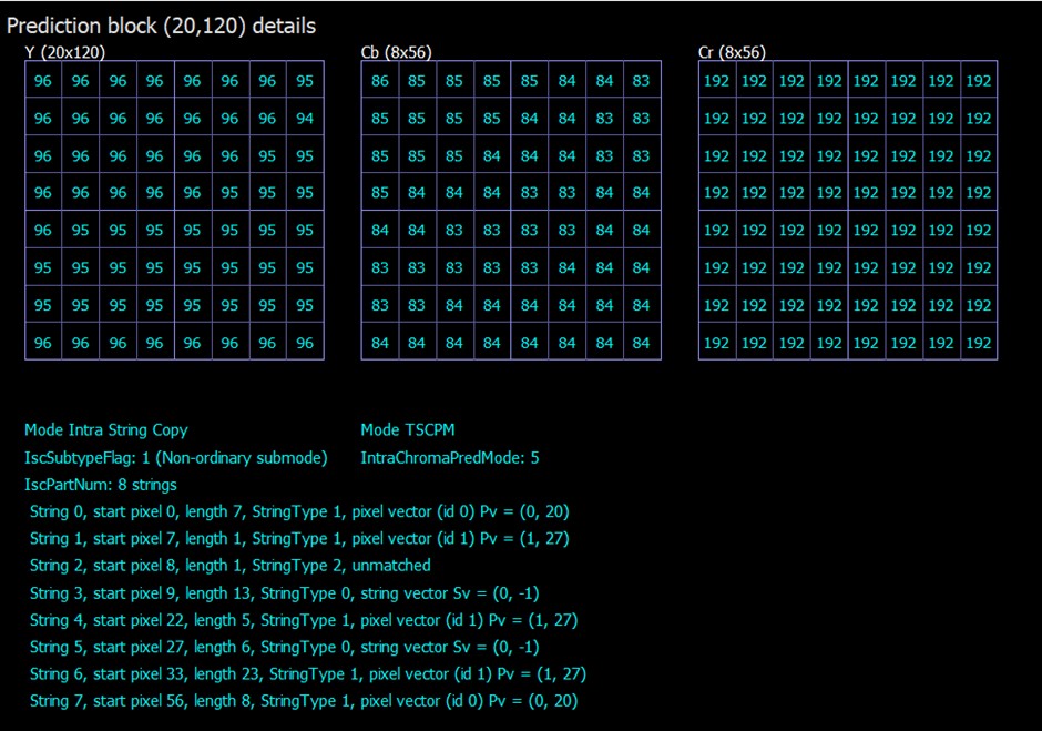
In Transform mode, the transform trees and accompanying residual signal of the picture can be seen. As in Prediction mode, the CU boundaries are shown with blue lines. The transform splits, when present, are indicated with yellow lines. QP values of each CU are shown in the lower-left corner. Luma coefficients are shown in the upper-left corner, chroma coefficients in the upper-right corner.
If the "Pic" button is turned on, the raw residual signal is shown in the image form. Transform values of 0 result in flat grey, negative values are darker and positive values are brighter.
Clicking on TUs causes that TU to be selected with a blue surrounding box and its syntax elements (when present) to be displayed in the Block tab In Syntax Info panel located to the left.
Full details of a particular TU or a group of TUs can be viewed by making the TU selection and entering detail mode by right clicking or using the Details mode button at the bottom of the main panel. In this mode, the structure of the selected TU is drawn three times and shows three major steps in recovering the residual signal - Coefficient decode, Inverse quantization and Inverse transformation. These steps are displayed by selecting the corresponding tab located to the right of the main panel - Residuals for Inverse transformation, QuantCoeff Matrix for Inverse quantization, and CoeffMatrix for Coefficient decode. The following describes each of these steps:
In Reconstruction mode the reconstructed samples can be inspected prior to deblocking. As with Prediction/Transform mode, CU boundaries are shown with blue lines. The Info button allows to select the following views:
Clicking on TUs causes that TU to be selected with a purple surrounding box and its syntax elements (when present) to be displayed in the Block tab In Syntax Info panel located to the left.
Full details of a particular TU or a group of TUs can be viewed by making the TU selection and entering detail mode by right clicking or using the Details mode button at the bottom of the main panel. In this mode, the structure of the selected TU is drawn three times and shows three major steps in recovering the residual signal.
Loop Filter mode shows all edges processed by deblocking filter. The edges shown are for the luma deblocking process and are color coded in the following manner:
Clicking on TUs causes that TU to be selected with a purple surrounding box and its syntax elements (when present) to be displayed in the Block tab In Syntax Info panel located to the left.
The deblocked sample values can be inspected directly in Details. As with Reconstruction Details, the inspected area can consist of one or more CUs. Sample values are indicated in yellow if they were modified by the deblocking process. Sample values that cannot be modified due to pcm_flag or cu_transquant_bypass_flag are indicated in red. Filtered edges belonging to the selected CU are shown in thick dashed lines, color coded the same way as in the non-detail mode. Each edge can be selected and clicked, bringing up a window showing the input values to the edge filter. Note that these values may differ from the reconstructed samples for horizontal edges, as they may have been modified by a vertical edge filter. Additionally, the boundary strength is displayed. Edges that were processed but ultimately not filtered (red colored) will indicate the reason. Typically it is due to the boundary strength being 0, the threshold condition not being met, or a slice/tile edge when those edges shouldn't be processed.
In SAO mode the SAO filter parameters assigned to each CTB are shown. The mode, and the associated four offsets for each component, are indicated with yellow text, and the merge_up / merge_left flags are indicated with an arrow. The CU quadtree boundaries are shown here as well.
The Info button allows to select the following views:
Entering detail mode on a selected CU will show all samples after being processed by the SAO filter. Sample values that were actually modified by the SAO operation are highlighted in yellow. Each sample can be clicked, bringing up a 3x3 window that shows the input values to the filter process. In the screenshot below, the 45-degree edge filter inputs are the samples to the lower left and upper right. Samples that cannot be modified by the filter are indicated in red.
In ESAO (Enhanced Sample Adaptive Offset) mode the ESAO filter parameters assigned to each TU are shown. The mode, and the associated four offsets for each component, are indicated with yellow text, and the merge_up / merge_left flags are indicated with an arrow. The CU quadtree boundaries are shown here as well.
The Info button allows to select the following views:
Entering detail mode on a selected CU will show all samples after being processed by the ESAO filter. Sample values that were actually modified by the SAO operation are highlighted in yellow.
In CSAO (Cross-Component Sample Adaptive Offset) mode the CCSAO filter parameters assigned to each TU are shown. The mode, and the associated four offsets for each component, are indicated with yellow text, and the merge_up / merge_left flags are indicated with an arrow. The CU quadtree boundaries are shown here as well.
The Info button allows to select the following views:
Entering detail mode on a selected CU will show all samples after being processed by the ESAO filter. Sample values that were actually modified by the SAO operation are highlighted in yellow.
In Adaptive Filter mode, for each TU, if available, the parameters of the adaptive loop filter are shown. The filter type and filter index for each component are indicated in yellow font.
Clicking on TUs causes that TU to be selected with a turquoise surrounding box and its syntax elements (when present) to be displayed in the Block tab In Syntax Info panel located to the left.
In Detail mode on a selected Block all samples processed by ALF filter are shown. Sample values that were modified by the ALF process are highlighted in yellow.
In YUV mode the final decoded sample values can be inspected without additional overlay data.
In Info Overlays Mode, an additional button appears in the Main View panel to the right. It gives an option of choosing between Heat, QpY, CoeffsY, PSNR, SSIM, and Statistics.
The Heat Map shows bits per CU density. CUs with more bits are brighter than CUs with fewer. Coloring of the bits range can be adjusted with a gradient tool on the right top corner.
[TBA] The QpY Map shows ..... Skip, None, values .... Blocks in purple, blocks in navy.
The Coeffs Y Map shows coefficient values. CUs with greater values are brighter than CUs with fewer. Coloring of the MV bits range can be adjusted with a gradient tool on the right top corner.
TBD
TBD
Statistics displays statistics of syntax elements in detail. Overall, the type of statistics displayed repeats the information that can be obtained in Syntax Info panel in Stats tab as it appears in the bottom window. However, more options of displaying statistics are available in Main View. For greater efficiency, Statistics in Main View panel can be displayed in parallel with Statistics in Syntax Info providing greater opportunities for analysis.
[insert pic of the menu]
Statistics in Main View panel can be operated by right-clicking the mouse which opens a context menu. The menu has the following options:
Add new Stat... - displays a new type of statistics. One can choose between CU Size, CU Mode, IntraChromeMode, IntraLumaMode, QpY, TU size
Delete Stat - deletes the statistics
Use percent - displays statistics in percentage
Apply percentage view to all - applies percentage view to all types of statistics displayed
Pie Chart - displays statistics as a pie chart
Bar Chart - displays statistics as a bar chart
Apply view mode to all - applies the selected mode (pie or chart) to all displayed statistics
Raw values - un-normalized numbers displayed as raw counts
Area normalized - normalized data weighted by area
Bits normalized - normalized data weighted by bits
Apply normalize method to all - applies the selected type of data (raw values, area normalized or bits normalized) to all displayed statistics
Picture stats - displays picture statistics
Stream stats - displays stream statistics (becomes available after running full stream analysis in Stream View)
Apply type of stats to all - applies the selected type of statistics (picture or stream) to all displayed statistics.
The pie/bar charts can be moved by dragging the mouse, and zoomed with the mouse scroll wheel.
The following sections describe all specific features available when loading an HEVC bitstream. The supported format of a bitstream is the raw bitstream with no surrounding container. Output from the publicly available HEVC reference software HM is in this format and can be opened directly. VQ Analyzer supports Main, Main 10, and Main Still Picture profiles, HEVC RExt profiles (including SCC), SHVC profile and HEVC MultiView profiles. Sequences that go beyond the profile limits maybe be supported as well.
Use Mode menu to see available modes.
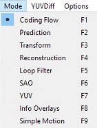
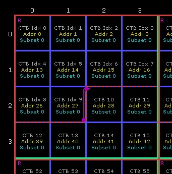
The coding flow mode gives a visual overview of the ordering of CTBs in the stream, and some information about the decoding process. The blue grid shows the boundaries of the CTBs in the picture. Each CTB contains 3 values:
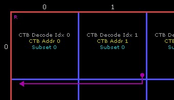
This mode shows the PUs in each CU. CU quad tree splits are indicated with blue lines, which get darker as the split depth increases. When a CU split is implied by HEVC and not directly coded in the bitstream, the split lines are dashed.
Intra modes are indicated with green colors, and directional modes also show an arrow indicating the prediction direction. In the lower right corner of an intra PU the chroma mode is indicated in a darker green. When the prediction shape is not the same as the CU size, the prediction unit shapes are shown with green lines for intra blocks, cyan for inter blocks. Dashed green lines in intra blocks means the PU was split along with the transform tree.
Inter PUs are indicated with cyan colors showing the PU splits and mode. Additionally, skipped blocks are shaded with a lined texture. An inter PU is Skip, AMVP or Merge mode. The L0 motion vectors are drawn with an orange color, the L1 motion vectors (B slices only) are drawn with a purple color. The MV value is shown in the lower left corner along with the reference index.
Clicking a PU will select it, and the syntax elements used to code it and the CU it belongs to are displayed in the CU tab on the left. Clicking repeatedly on the same PU will cycle through the CU hierarchy, showing the parent and child relationship.
Below is shown Prediction mode on a zoomed-in selection along the top edge of a picture. The selected CU is surrounded with a pink box while the selected PU is surrounded with a yellow box.
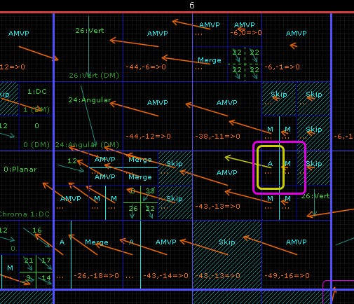
In Prediction mode, the sample values of a particular PU can be viewed in detail.
Intra PUs are displayed in green, and the left, upper-left and above prediction arrays are drawn adjacent. Luma blocks show 3 versions of the predictions arrays. From furthest out to in, they represent the arrays in 3 steps:
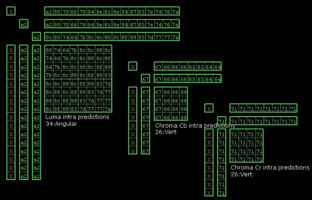
Inter PUs are displayed in cyan (turquoise). Each prediction sample can be clicked to display a window that contains the 8x8 or 4x4 sample array for luma or chroma respectively that are the inputs to the motion compensation filter for the selected pixel. In the case of a bi-directional PU, both arrays are shown the L0/L1 colors of orange/purple. Clicking the selected sample again or outside the PU closes this window. Underneath the prediction array values the motion vector predictor lists are displayed. In merge mode, the merge list is shown with the L0 predictor in orange and the L1 predictor in purple. An arrow indicates the merge candidate that is chosen by the bitstream (merge_idx).
When the inter PU does not code motion vectors in merge mode, it is considered AMVP mode (Advance Motion Vector Prediction). The 2-entry list for each motion vector (L0 and/or L1) is shown and the selected predictor is indicated with an arrow.
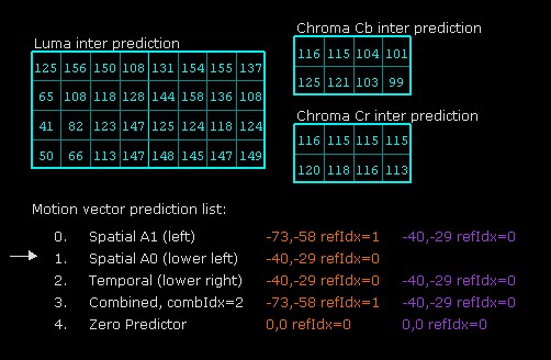
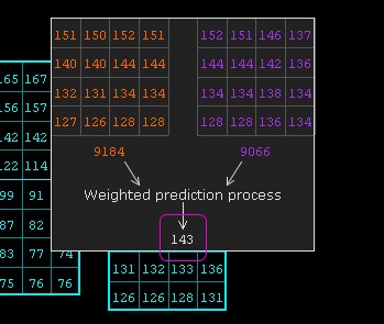
For HEVC screen content coding stream there is special detail mode exist -- Palette mode. In this mode VQ Analyzer shows palette predictor, currently used palette, coded indices, resulting indices and final pixel values.
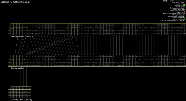
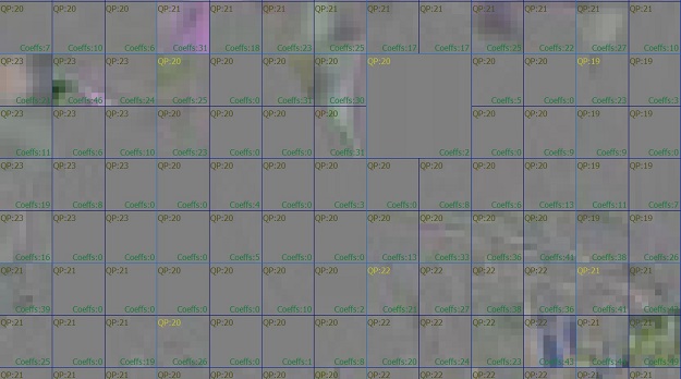
In Transform mode the transform trees and accompanying residual signal of the picture can be seen. As in Predictions mode, the CU boundaries are shown with blue lines. The transform splits, when present, are indicated with yellow lines. A dashed yellow line indicates that the TU split was implied. The QP values of each CU are shown in the upper-left corner. The number of non-zero coefficients is shown in the left-bottom corner. When this value is bright yellow, it means that a delta-QP was coded in the bitstream during the decode of that particular CU. Otherwise the number is dark. When DQP is enabled by the PPS, this helps visualize the DQP coding depth (diff_cu_qp_delta_depth). TUs that have transform_skip_flag set are shaded. CUs that are PCM coded are marked with "PCM" in white, and CUs that have cu_transquant_bypass_flag set have a white X through them.
If the "Pic" button is turned on, the raw residual signal is shown in image form. Transform values of 0 result in flat grey, negative values are darker and positive values are brighter.
Clicking on TUs causes that TU to be selected with a blue surrounding box and its syntax elements (when present) to be displayed in the TU tab of the left panel. Clicking a TU repeatedly causes the selection to move up and cycle though the TU, then CU quadtree hierarchy. Note that when the selected TU is a 4x4, the chroma coefficients are coded one level up in the TU hierarchy since HEVC doesn't specify a 2x2 chroma TU. So to view chroma TU syntax when the luma TU is 4x4, click the luma TU twice to move up to the 8x8 level where the chroma syntax is decoded.
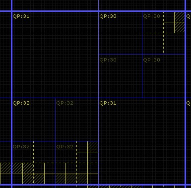
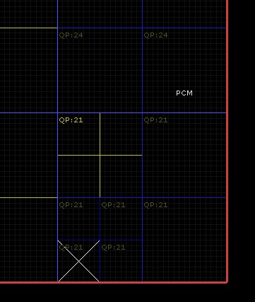
To view the full details of a particular TU or group of TUs, make the TU selection and enter detail mode by right clicking or using the detail mode button at the bottom of the main panel. In this mode the selected TU structure is drawn three times, arranged in a column from top to bottom, showing the 3 major steps in recovering the residual signal:
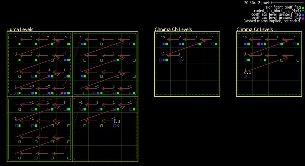
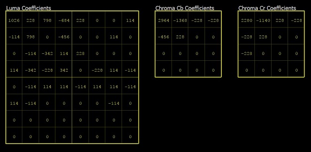
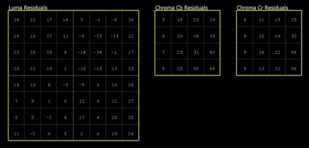
In Reconstruction mode the reconstructed samples can be inspected prior to deblocking. As with Prediction/Transform mode, CU boundaries are shown with blue lines. CUs that have at least one TU with non-zero coefficients are marked with "Non-zero CBF". PCM-coded CUs are indicated with "PCM" in white.
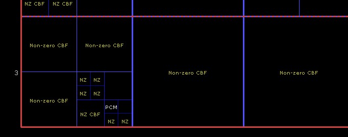
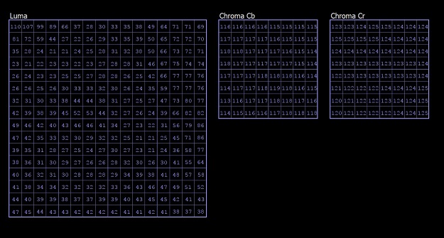
Loop Filter mode shows all edges processed by the deblocking filter as described in the MB. Boundaries are not displayed in this mode, however MB selection still functions as in the other modes. Edges shown are for the luma deblocking process and are color coded in the following manner:
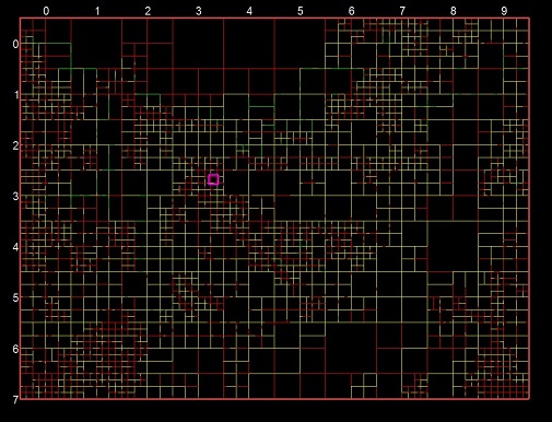
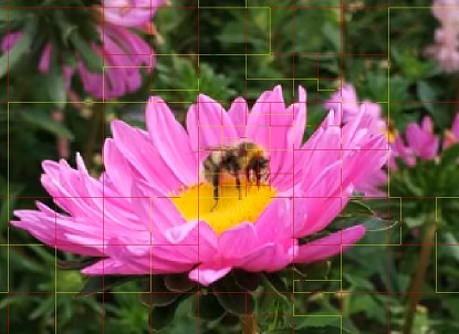
The deblocked sample values can be inspected directly in detail mode. As with Reconstruction Details, the inspected area can consist of one or more CUs. Sample values are indicated in yellow if they were modified by the deblocking process. Sample values that cannot be modified due to pcm_flag or cu_transquant_bypass_flag are indicated in red. Filtered edges belonging to the selected CU are shown in thick dashed lines, color coded the same way as in the non-detail mode. Each edge can be selected and clicked, bringing up a window showing the input values to the edge filter. Note that these values may differ from the reconstructed samples for horizontal edges, as they may have been modified by a vertical edge filter. Additionally, the boundary strength is displayed. Edges that were processed but ultimately not filtered (red colored) will indicate the reason. Typically it is due to the boundary strength being 0, the threshold condition not being met, or a slice/tile edge when those edges shouldn't be processed.
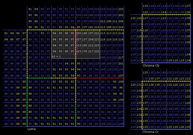
In SAO mode the SAO filter parameters assigned to each CTB are shown. The mode, and the associated four offsets for each component, are indicated with yellow text, and the merge_up / merge_left flags are indicated with an arrow. The CU quadtree boundaries are shown here as well.
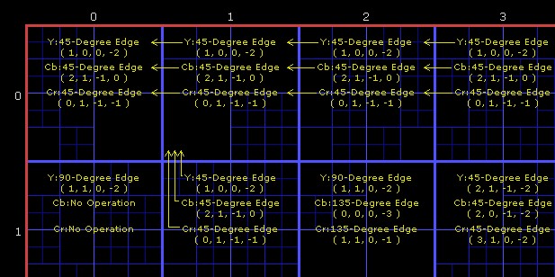
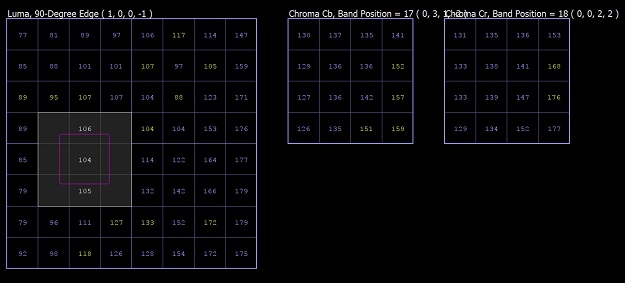
YUV mode allows the user to inspect the final decoded sample values, without additional overlay data.
There are a number of overlays that provide additional information about the picture that you're currently investigating. When you switch to "Info Overlays" mode, several additional submenus will appear in the bottom-left panel of info window.
You can switch now between additional modes with the drop down menu on the right. PSNR and SSIM modes are enabled if you have loaded a reference YUV file.
The heat map mode gives a visual representation of how the compressed bits of the picture are distributed spatially. Blocks with more bits per pixel are brighter than blocks with fewer. By zooming in, actual CU sizes in bits will be displayed as soon as its size is in the borders of the CU. By default, this mode also shows the CU quadtree boundaries in blue. It may be useful to turn off this overlay using the "Info" button on the lower left of the main panel. Heat Map does not offer a detail mode.
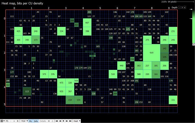
Maximum shown CU depth level can be restricted with the "Depth" on-screen control. Click on '+' and '-' to choose your required depth level.
The gradient used to display the heat map can also be edited:
The MV Map show mv bits per CU. CUs with more mv bits are brighter than CUs with fewer. Coloring of the MV bits range can be adjusted with a gradient tool on the right top corner.
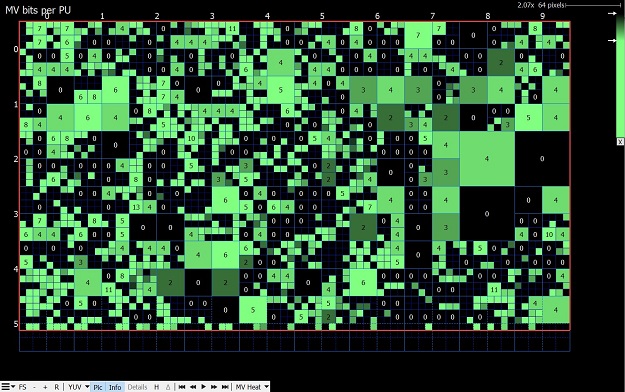
The QP Map shows per-block QP. CUs with bigger QP are brighter than CUs with smaller QP. Coloring of the QP range can be adjusted with a gradient tool on the right top corner. On the 'skip' blocks, the QP does not change and they are colored red.
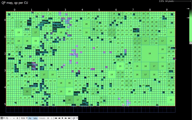
The PSNR map shows per-pixel PSNR values, normalized on block size. To enable this mode you have to load the reference YUV file via the DebugYUV menu. The value is calculated per block. A bigger value is shown with a brighter color. The color range can be adjusted with the gradient tool on the right top corner. If the block has no difference to the reference YUV, a letter 'e' is shown, standing for 'exact match'.
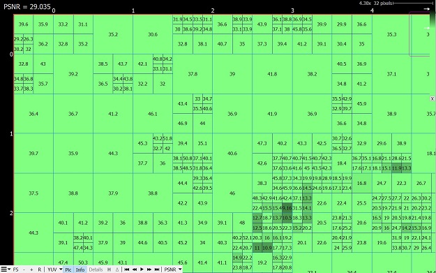
The SSIM map shows per-pixel SSIM values, normalized on CU size. To enable this mode you have to load a reference YUV file via the DebugYUV menu. The value is calculated per CU. Bigger values have a brighter white color.
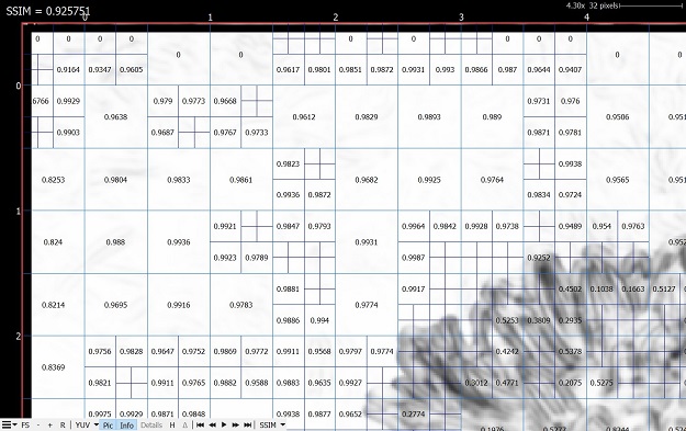
The PU Type overlay shows a color map of their types. Intra blocks are colored in red, inter skip is yellow, inter merge is in green, and inter is blue. The legend on the right top corner show color types for blocks. The gradient band lets you adjust transparency when the Pic switch is on.
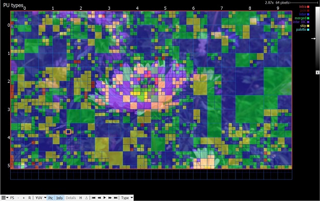
PU reference indices shows reference indices for each PU. Orange color shows L0 reference index and purple color is for L1 reference index. When a PU has only one reference missing, the reference index is displayed with dash. For blocks with no reference indices, nothing is shown.
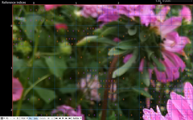
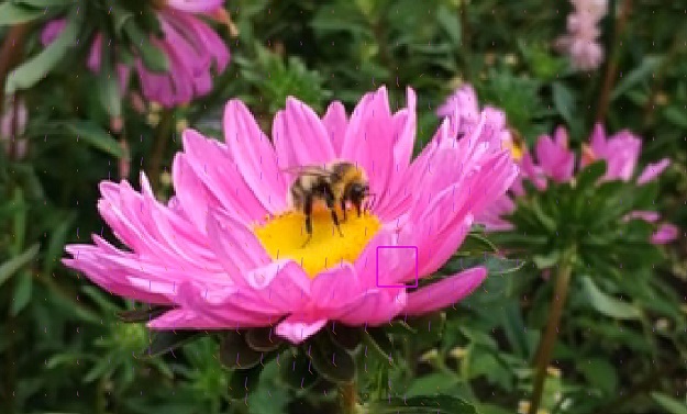
Simple Motion mode offers a way to quickly view the modes and motion of any picture at a glance. No overlays are present except a colored dot showing information about the PU's mode. Green dots indicate intra prediction, and purple/orange L0/L1 motion vectors for inter prediction are drawn as simple lines. When the motion vector is very small, a dot is drawn instead so that the mode is still easy to identify. When a motion vector does not point to the 0-th index of its respective list, the vector is drawn using a dashed line.
The following sections describe all specific available features when loading a VP9 bitstream. The bitstream must be containerized with either the WebM or IVF container format. The publicly available VP9 reference software can output both formats. Raw uncontainerized bitstreams are presently not supported due to the nature of the VP9 standard; there is no way to determine where each frame starts without doing a full decode of the sequence.
Use the Mode menu to see available modes.
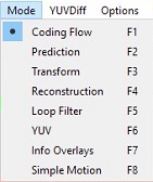
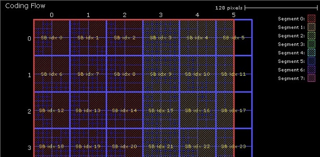
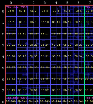
Coding flow mode gives an overview of the way the frame is constructed. Each superblock's decode index is shown in yellow and block-partioning is indicated with blue boundaries. Tile boundaries, when present, are shown with thick green lines and the tile size as coded in the bitstream is shown at the top left of each tile that has a size coded. When segmentation is enabled, each segment is shaded with a unique color. No detail mode is available.
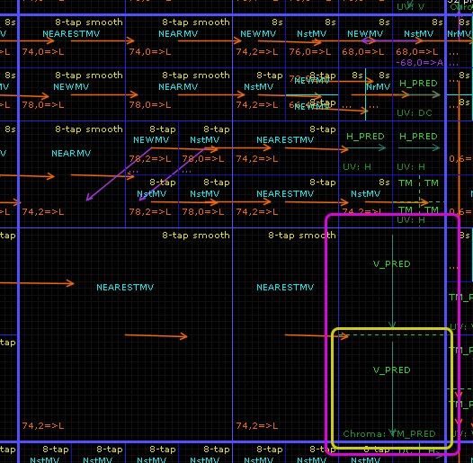
This mode shows the details of the prediction blocks in the frame. Block splits are indicated with blue lines, the selected block is surrounded with a pink box and the selected prediction block is surrounded with a yellow box. When a prediction block is selected, the syntax used to code it is displayed in the Block tab of the Left Panel. Clicking a block repeatedly will navigate the recursive block hierarchy.
Intra prediction block contains the intra luma mode in bright green, and the chroma intra mode in dark green near the bottom of the block. When the intra prediction operation is split due to the size of the transform blocks, the intra split boundaries are indicated with dashed green lines. Directional intra luma modes also contain a turquoise arrow indicating the prediction direction.
Inter prediction blocks show the inter mode in cyan, the first motion vector in orange and the second motion vector in purple. The motion vector value is in units of 1/8^th^ pixels. After the motion vector value the reference frame it points to is indicated with a single letter: L for Last, G for Golden and A for AltRef. The motion compensation filter type that applies to the prediction block is indicated in yellow near the top right corner of the block.
Entering detail mode on a selected prediction block allows the sample values of the prediction process to be viewed directly.
Intra-predicted blocks display the intra prediction process of each component. The left, above-left and above reference sample arrays are shown as well.
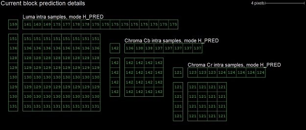
Inter-predicted blocks show the filtered prediction samples arrays of each component, the predictor list used for motion vector prediction (for each motion vector) and the filter type applied. To the left of the prediction sample arrays the impulse response of the applied filter is drawn (mostly decoratively). Each prediction sample can be clicked to display a window that contains the 8x8 or 4x4 sample array for luma or chroma respectively that are the inputs to the motion compensation filter for the selected pixel. The applicable filter phases are also indicated. In the case of compound prediction, both arrays & phase sets are shown with the first/second colors of orange/purple. Clicking the selected sample again or outside the block closes this window.
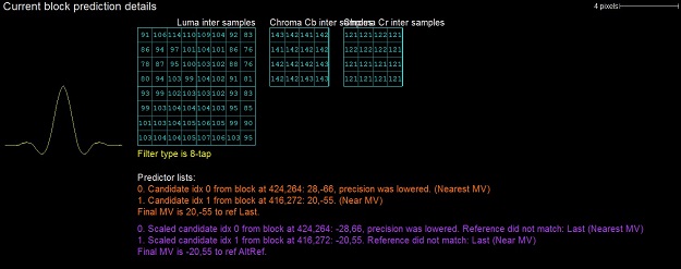
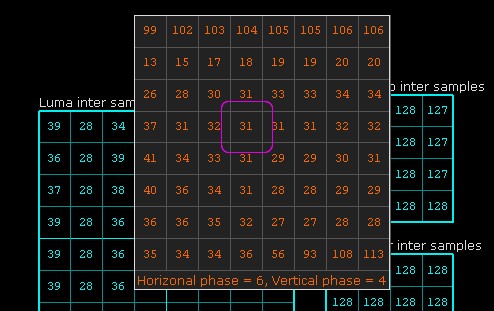
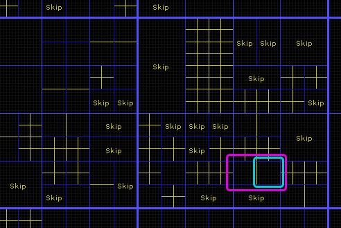
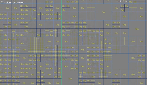
Transform mode allows for the inspection of the transform structure of each block. Block boundaries are displayed in blue, the currently selected block is outlined with a pink box and the selected transform block is outlined with a blue box. Blocks that code no residual signal are indicated with "Skip" in yellow. Blocks that use a transform size that is smaller than the block's own size show the transform boundaries within the block in yellow.
Clicking a particular transform block causes the syntax elements used to decode it to be visible in the "TX" tab of the Left Panel.
The residual image itself can be shown using the "Pic" button on the bottom button strip. Residual values of 0 are flat gray, negative values are darker and positive values are brighter.
The VQ Analyzer shows the number of non-zero coefficients with "Coeffs: 2" label on the corresponding block.
To view the full details of the transform blocks belonging to a particular block, select a transform block and enter detail mode by right clicking or using the detail mode button at the bottom of the main panel. The currently selected transform block is highlighted with the sample grid. The transform structure of the selected block is drawn three times, and arranged in a column from top to bottom, showing the 3 major steps in recovering the residual signal:
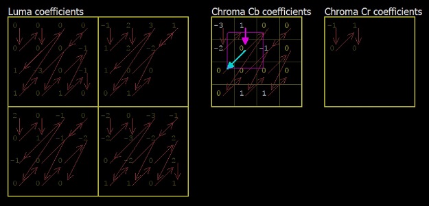
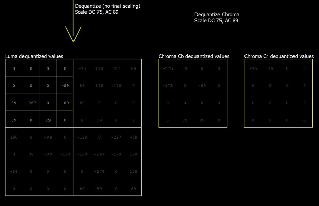
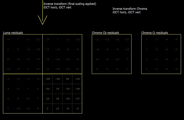
In Reconstruction mode, the reconstructed samples can be inspected prior to loop filtering. As with Prediction/Transform mode, block boundaries are shown with blue lines. Blocks with no coefficients are marked with "Skip" in white.
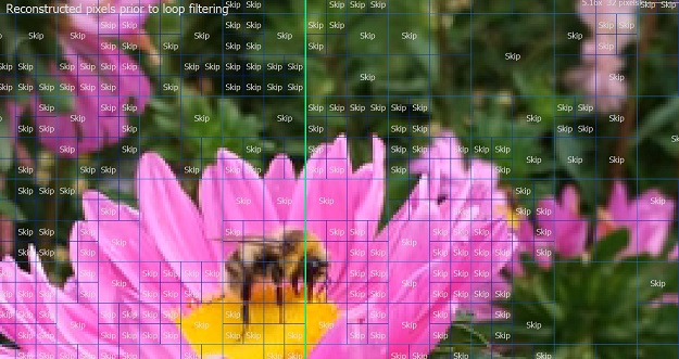
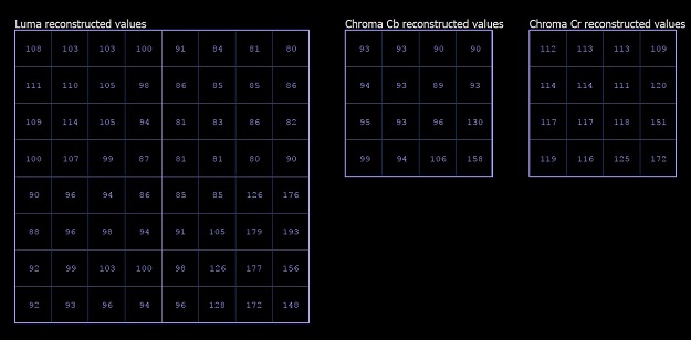
Loop filter mode shows all processed edges in the frame. Edges are 1 sample high/tall, and are color coded as follows:
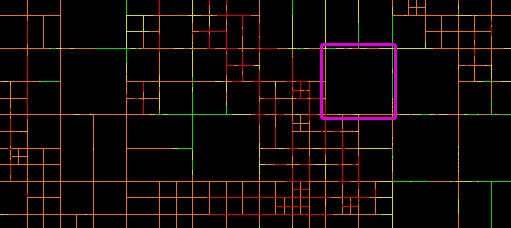
The filtered sample values can be inspected directly in detail mode. As with Reconstruction Details, the inspected area can consist of one or more blocks. Sample values are indicated in yellow if they were modified by the deblocking process. Samples to the left and above the current block needed for the filter are shown as well. Filtered edges belonging to the selected blocks are shown in thick dashed lines, color coded the same way as in non-detail mode. Each edge can be selected and clicked, bringing up a window showing the input values to the edge filter. Note that these values may differ from the reconstructed samples, as they may have been modified by an earlier edge filter.
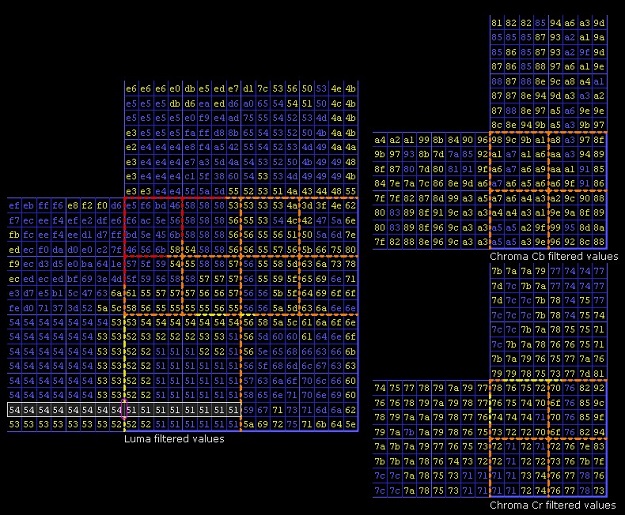
YUV mode allows the user to inspect the final decoded sample values, without additional overlay data.
There are a number of overlays that provide additional information about the picture that you're currently investigating. When you switch to "Info Overlays" mode, several additional submenus will appear in the bottom-left panel of info window.
You can switch now between additional modes with the drop down menu on the right. PSNR and SSIM modes are enabled if you have loaded a reference YUV file.
The heat map mode gives a visual representation of how the compressed bits of the picture are distributed spatially. Blocks with more bits per pixel are brighter than blocks with fewer. By zooming in, actual CU sizes in bits will be displayed as soon as its size is in the borders of the CU. By default, this mode also shows the CU quadtree boundaries in blue. It may be useful to turn off this overlay using the "Info" button on the lower left of the main panel. Heat Map does not offer a detail mode.
Maximum shown CU depth level can be restricted with the "Depth" on-screen control. Click on '+' and '-' to choose your required depth level.
The gradient used to display the heat map can also be edited:
Block Type overlay shows a color map of block types. Intra blocks are colored in red, inter skip are yellow colored and inter are in blue.
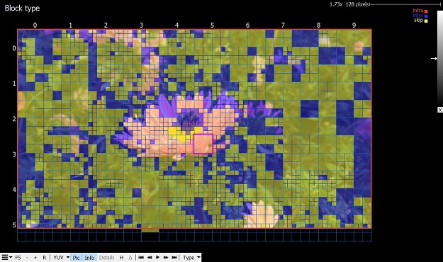
Efficiency map mode shows visually how efficient the arithmetic coding of each block is. Blocks with more bools per bits are brighter than blocks with less. By default this mode also shows the block boundaries in blue. It may be useful to turn off this overlay using the "Info" button on the lower left of the main panel. Efficiency Map does not offer a detail mode.
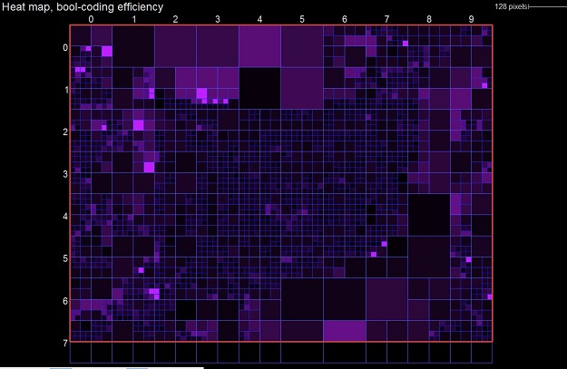
The PSNR map shows per-pixel PSNR values, normalized on block size. To enable this mode you have to load the reference YUV file via the DebugYUV menu. The value is calculated per block. A bigger value is shown with a brighter color. The color range can be adjusted with the gradient tool on the right top corner. If the block has no difference to the reference YUV, a letter 'e' is shown, standing for 'exact match'.
Simple Motion mode offers a way to quickly view the modes and motion of any picture at a glance. No overlays are present except a colored dot showing information about the PU's mode. Green dots indicate intra prediction, and purple/orange L0/L1 motion vectors for inter prediction are drawn as simple lines. When the motion vector is very small, a dot is drawn instead so that the mode is still easy to identify. When a motion vector does not point to the 0-th index of its respective list, the vector is drawn using a dashed line.
The following sections describe all available features when loading a AV1 bitstream. The bitstream must be containerized with either the WebM or IVF container format. The publicly available AV1 reference software can output both formats. Raw, uncontainerized bitstreams are presently not supported due to the nature of the AV1 standard; there is no way to determine where each frame starts without doing a full decode of the sequence.
Use the Mode menu to see available modes.
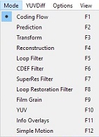

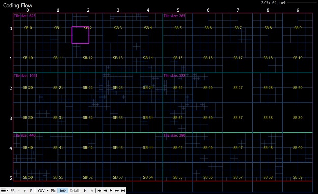
Coding flow mode gives an overview of the way the frame is constructed. Each superblock's decode index is shown in yellow and block-partioning is indicated with blue boundaries. Tile boundaries, when present, are shown with thick green lines and the tile size, as coded in the bitstream, is shown at the top left of each tile that has a size coded. When segmentation is enabled, each segment is shaded with a unique color. No detail mode is available.
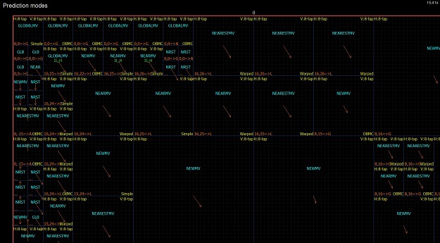
This mode shows the details of the prediction blocks in the frame. Block splits are indicated with blue lines, the selected block is surrounded with a pink box and the selected prediction block is surrounded with a yellow box. When a prediction block is selected, the syntax used to code it is displayed in the Block tab of the Left Panel. Clicking a block repeatedly will navigate the recursive block hierarchy.
Intra prediction blocks contain the intra luma mode in bright green, and the chroma intra mode in dark green near the bottom of the block. When the intra prediction operation is split due to the size of the transform blocks, the intra split boundaries are indicated with dashed green lines. Directional intra luma modes also contain a turquoise arrow indicating the prediction direction.
Inter prediction blocks show the inter mode in cyan, the first motion vector in orange and the second motion vector in purple. The motion vector value is in units of 1/8th pixels. After the motion vector value, the reference frame it points to is indicated with a single letter: L for Last, G for Golden and A for AltRef. The motion compensation filter type that applies to the prediction block is indicated in yellow near the top right corner of the block. If inter mode contains intrainter prediction intra mode, this will be written under inter mode in bright green.
The VQ Analyzer shows horizontal and vertical filtering separately for each block on the left and right top corners accordingly. Motion type is shown in the bottom right corner of the block.
Entering detail mode on a selected prediction block allows the sample values of the prediction process to be viewed directly.
Intra-predicted blocks display the intra prediction process of each component. The left, above-left and above reference sample arrays are shown as well.
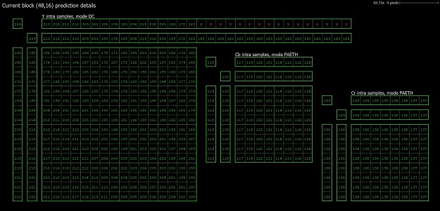
Inter-predicted blocks show the filtered prediction samples arrays of each component, the predictor list used for motion vector prediction (for each motion vector) and the filter type applied.
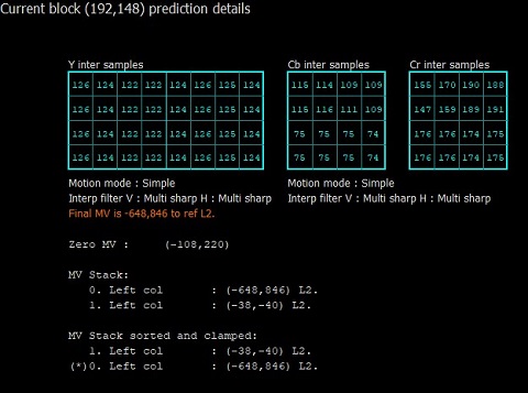
Zero MV - motion vector mv representing global motion for this block
MV Stack: motion vectors after Find MV Stack Process (This process constructs an array RefStackMv containing motion vector candidates).
MV Stack Sorted: motion vectors from MV Stack after sorting, extra search and clamping processes.
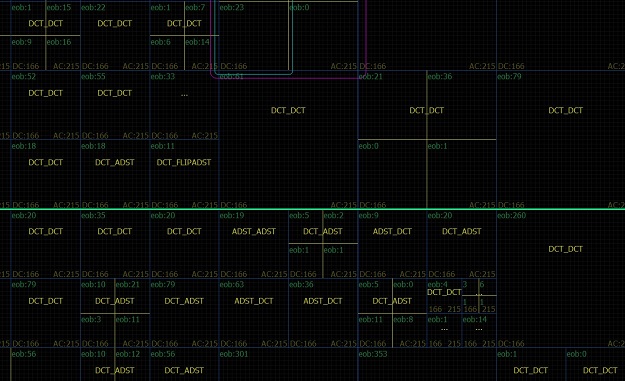
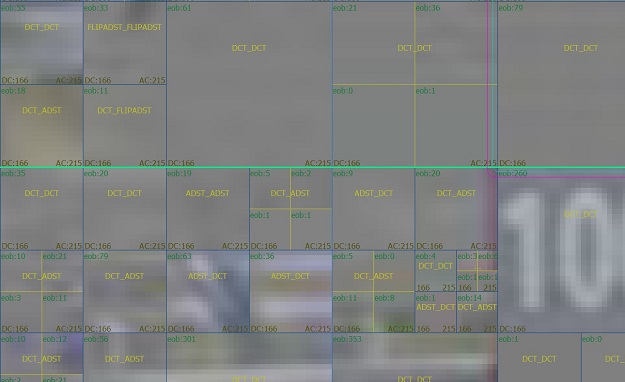
Transform mode allows inspection of the transform structure of each block. Block boundaries are displayed in blue, the currently selected block is outlined with a pink box and the selected transform block is outlined with a blue box. Blocks that code no residual signal are indicated with "Skip" in yellow. Blocks that use a transform size that is smaller than the block's own size show the transform boundaries within the block in yellow.
The residual image itself can be shown using the "Pic" button on the bottom button strip. Residual values of 0 are flat gray, negative values are darker and positive values are brighter.
To view the full details of the transform blocks belonging to a particular block, select a transform block and enter detail mode by right clicking or using the detail mode button at the bottom of the main panel. The currently selected transform block is highlighted with the sample grid. The transform structure of the selected block is drawn three times, arranged in a column from top to bottom, showing the 3 major steps in recovering the residual signal:
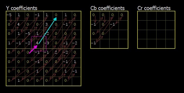
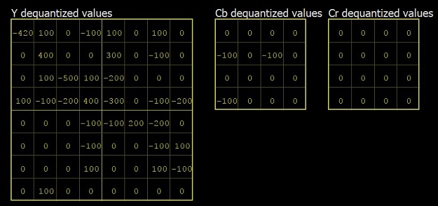
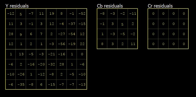
In Reconstruction mode the reconstructed samples prior to loop filtering can be inspected. As with Prediction/Residual mode, block boundaries are shown with blue lines. Blocks with no coefficients are marked with "Skip" in white.
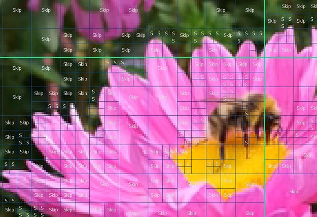
In detail mode, the reconstructed sample values can be inspected. The selection may be a single block, or a group of blocks up to and including the entire encompassing super-block.
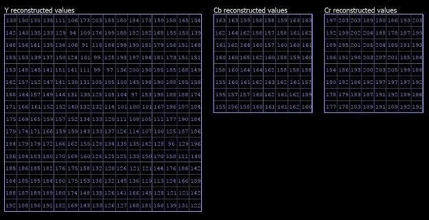
Loop filter mode shows all the processed edges in the frame. Edges are 1 sample high/tall, and are color coded as follows:

The filtered sample values can be inspected directly in detail mode. As with Reconstruction Details, the inspected area can consist of one or more blocks. Sample values are indicated in yellow if they were modified by the deblocking process. Samples to the left and above the current block need for the filter are shown as well. Filtered edges belonging to the selected blocks are shown in thick dashed lines, color coded the same way as in non-detail mode. Each edge can be selected and clicked, bringing up a window showing the input values to the edge filter. Note that these values may differ from the reconstructed samples, as they may have been modified by an earlier edge filter.
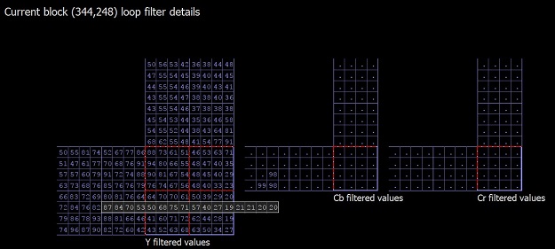
CDEF mode shows all the processed blocks in the frame. There are three parameters shown for each block: level, strength and CDEF direction.
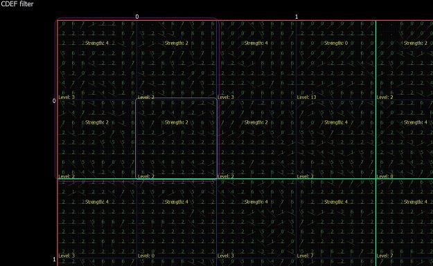
The filtered sample values can be inspected directly in detail mode. As with Reconstruction Details, the inspected area can consist of one or more blocks. Sample values are indicated in yellow if they were modified by the CDEF process.
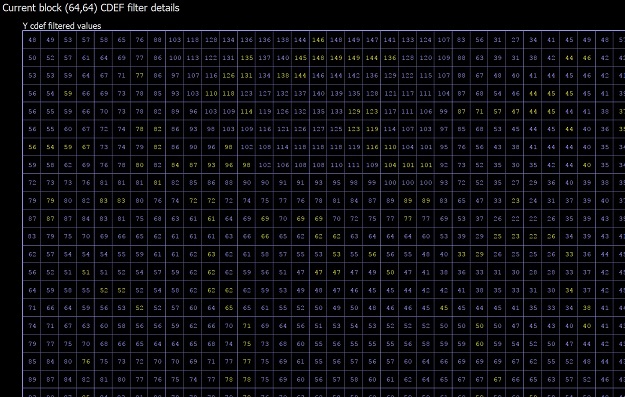
If superres is enabled, in SuperRes Filter mode upscaled bloсks can be expected. Scaling factor is shown in top left. Upscaled blocks splits are indicated with grey lines. By left mouse click, block 8x8 or 64x64 pixels for viewing in detail can be selected.
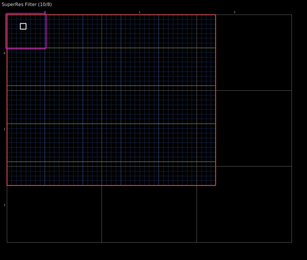
If superres is enabled, in SuperRes Filter detail mode upscaled pixels can be expected. By click on a pixel, superres params are shown. For 64x64 blocks above and bottom stripes are present.
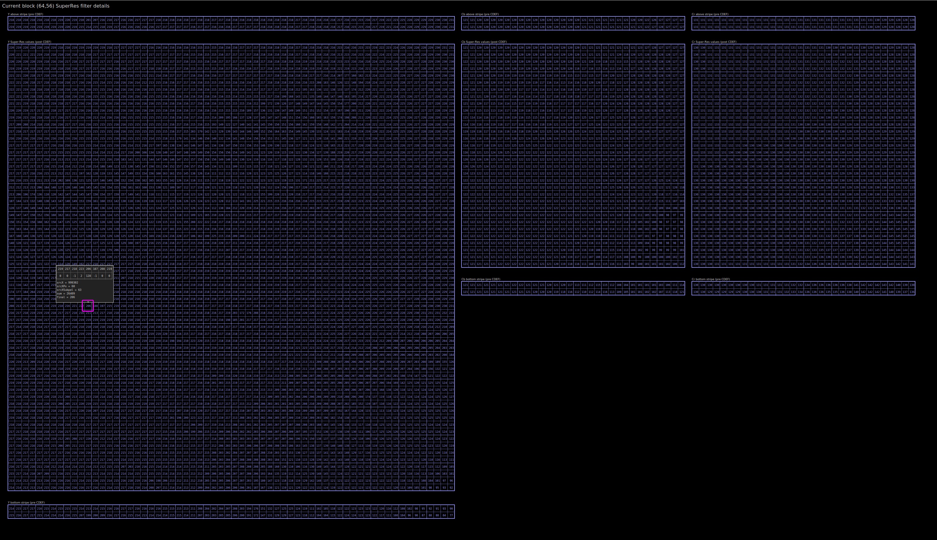
Loop restoration filter shows all processed blocks in the frame. The information on each block shows the filter type and the size of the block itself.
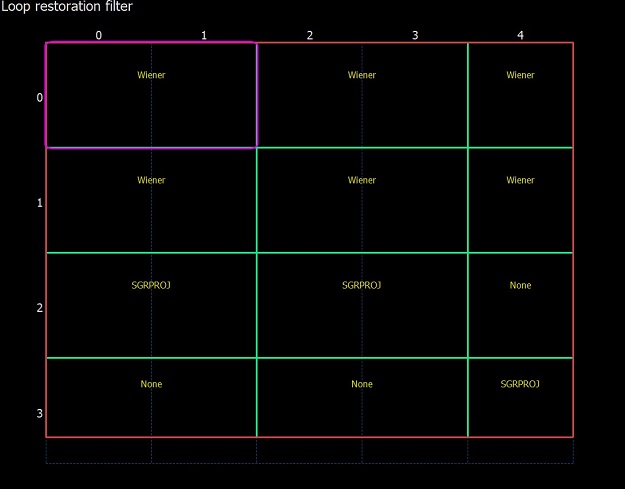
The analyzer shows more filter parameters in detail mode.
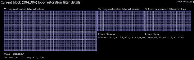
If film grain is enabled, in Film Grain Pixels mode samples after film grain synthesis process can be expected. 32x32 blocks can be selected for detailed view.
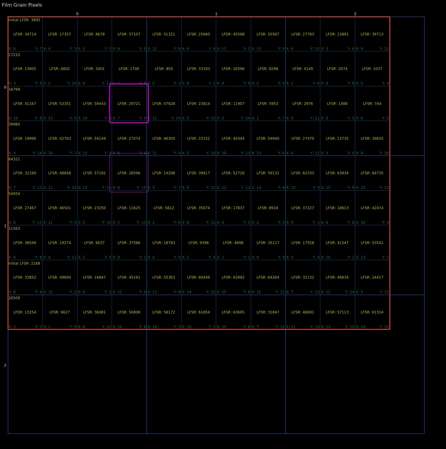
Entering detail mode on a selected 32x32 block will show all samples after the film grain synthesis process. Sample values that were actually modified by the film grain synthesis process are highlighted in yellow. Each sample can be clicked, bringing up a grey window with formula for calculating value.
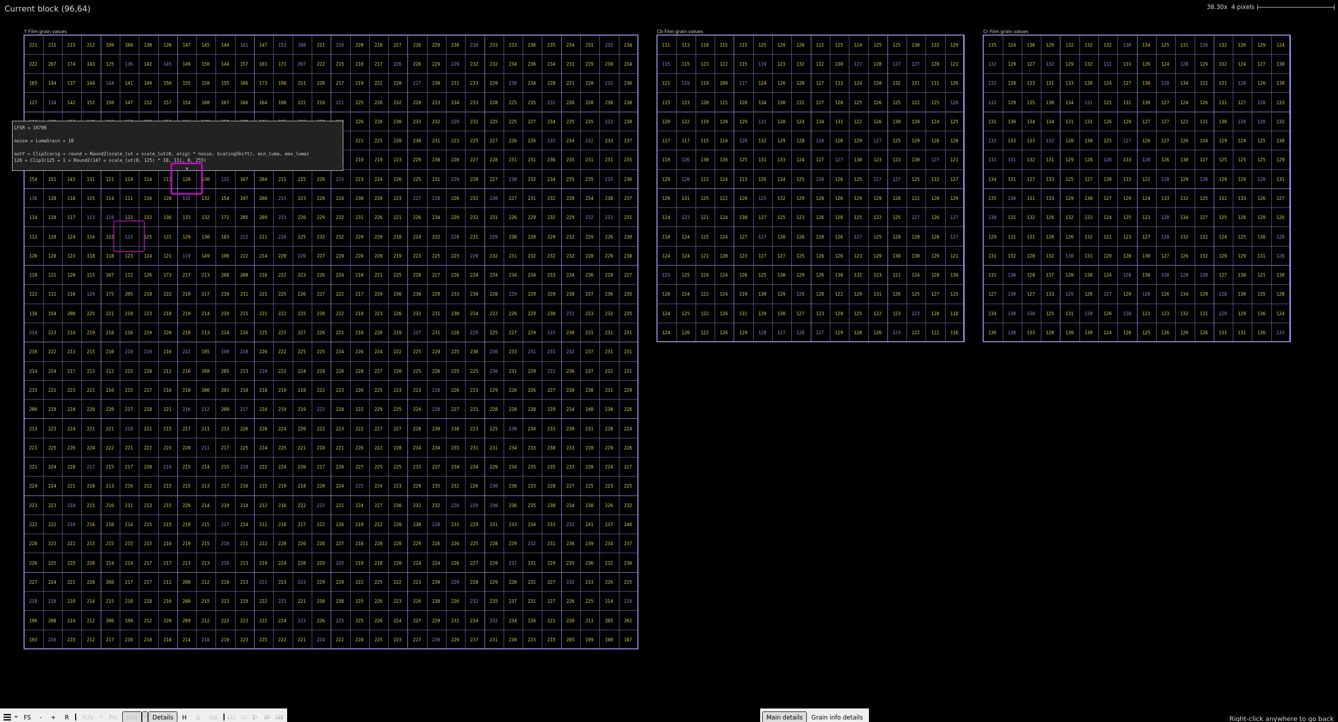
In the bottom by click on "Grain info details" LumaGrain, CbGrain and CrGrain arrays can be expected. Each sample can be clicked, bringing up a gray window with formula for calculating value.
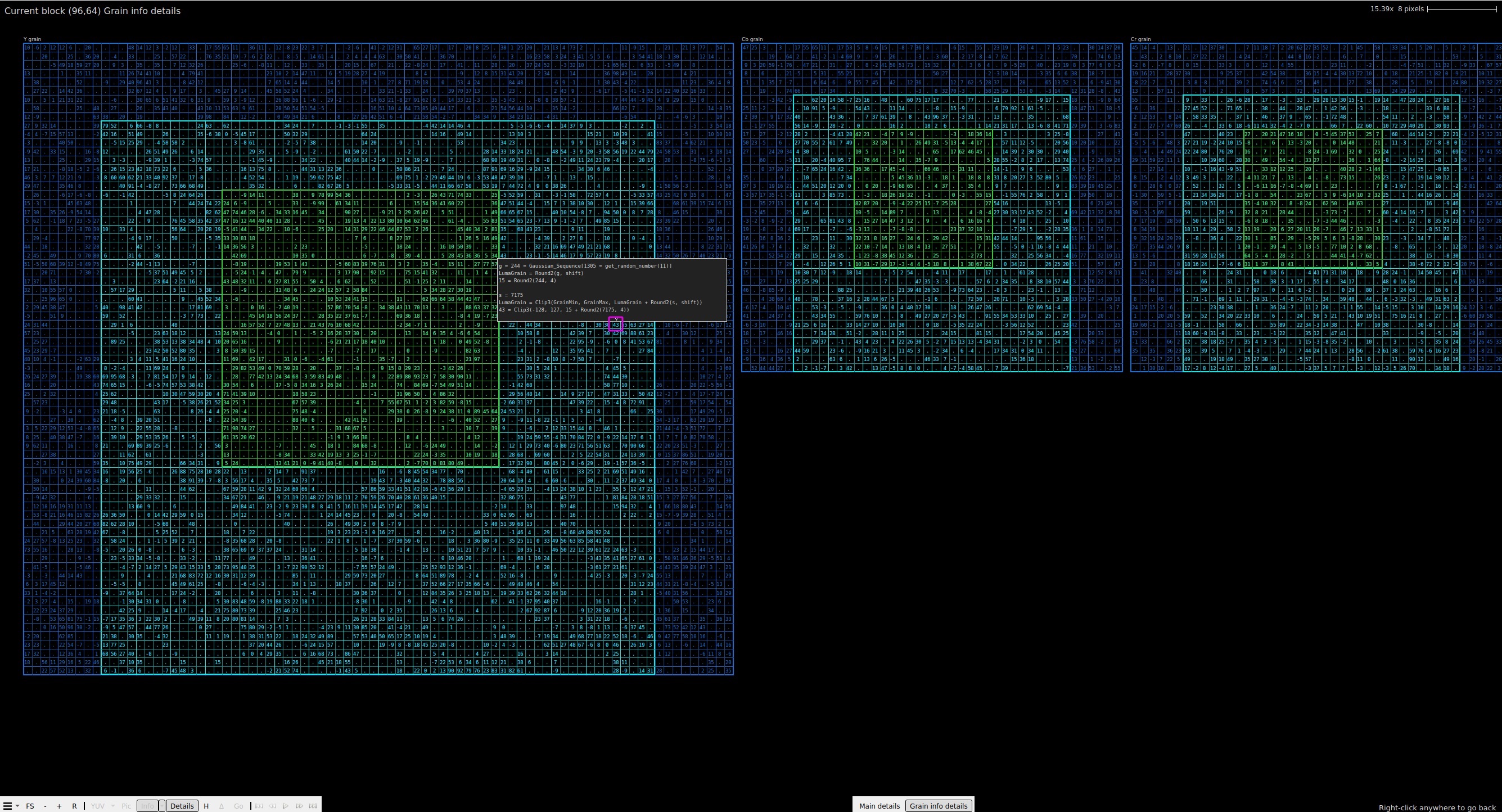
YUV mode allows the user to inspect the final decoded sample values, without additional overlay data.
There are a number of overlays that provide additional information about the picture that you're currently investigating. When you switch to "Info Overlays" mode, several additional submenus will appear in the bottom-left panel of info window.
You can switch now between additional modes with the drop down menu on the right. PSNR and SSIM modes are enabled if you have loaded a reference YUV file.
The heat map mode gives a visual representation of how the compressed bits of the picture are distributed spatially. Blocks with more bits per pixel are brighter than blocks with fewer. By zooming in, actual CU sizes in bits will be displayed as soon as its size is in the borders of the CU. By default, this mode also shows the CU quadtree boundaries in blue. It may be useful to turn off this overlay using the "Info" button on the lower left of the main panel. Heat Map does not offer a detail mode.
Maximum shown CU depth level can be restricted with the "Depth" on-screen control. Click on '+' and '-' to choose your required depth level.
The gradient used to display the heat map can also be edited:
Efficiency map mode shows visually how efficient the arithmetic coding of each block is. Blocks with more bools per bits are brighter than those with fewer. By default, this mode also shows the block boundaries in blue. It may be useful to turn off this overlay using the "Info" button on the lower left of the main panel. Efficiency Map does not offer a detail mode.

Block Type overlay shows a color map of the various types. Intra blocks are colored in red, inter skip are yellow colored and inter are in blue.
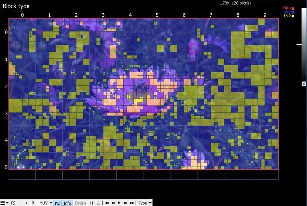
The PSNR map shows per-pixel PSNR values, normalized on block size. To enable this mode you have to load the reference YUV file via the DebugYUV menu. The value is calculated per block. A bigger value is shown with a brighter color. The color range can be adjusted with the gradient tool on the right top corner. If the block has no difference to the reference YUV, a letter 'e' is shown, standing for 'exact match'.
Simple Motion mode offers a way to quickly view the modes and motion of any picture at a glance. No overlays are present except a colored dot showing information about the PU's mode. Green dots indicate intra prediction, and purple/orange L0/L1 motion vectors for inter prediction are drawn as simple lines. When the motion vector is very small, a dot is drawn instead so that the mode is still easy to identify. When a motion vector does not point to the 0-th index of its respective list, the vector is drawn using a dashed line.
The following sections describe all available features when loading a MPEG-2 bitstream. The bitstream must be containerized with mpeg-2 container format.
Use the Mode menu to see available modes.
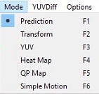
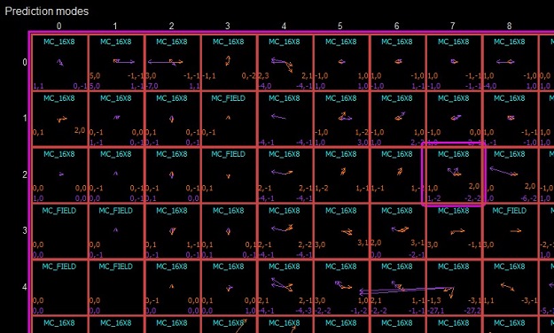
This mode shows the details of the prediction blocks in the frame. The selected block is surrounded with a pink box. When a prediction block is selected, the syntax used to code it is displayed in the Block tab of the Left Panel.
Intra prediction block contains the intra luma mode in bright green, and can contain so-called "concealment" motion vectors if they are present in bitstream.
Inter prediction blocks show the inter mode in cyan. Up to two pairs of MVs are drawn in a block. The left pair corresponds to the first field. The right one -- to the second one (if any). The forward motion vector in orange and the backward one in purple. The motion vector value is in units of 1/8^th^ pixels.
Entering detail mode on a selected prediction block allows the sample values of the prediction process to be viewed directly. No details mode is available for intra blocks.
Inter-predicted blocks display contains predicted values for luma and chroma components.
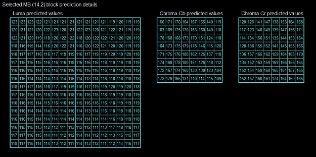
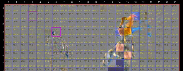
Transform mode allows the user to inspect the transform structure of each block. Block boundaries are displayed in blue, and the currently selected block is outlined with a pink box. Blocks that code no residual signal are indicated with "Skip" label.
Clicking a particular transform block causes the syntax elements used to decode it to be visible in the "MB" tab of the Left Panel.
The residual image itself can be shown using the "Pic" button on the bottom button strip. Residual values of 0 are flat gray, negative values are darker and positive values are brighter.
To view the full details of the transform blocks belonging to a particular block, selected a transform block and enter detail mode by right clicking or using the detail mode button at the bottom of the main panel. The currently selected transform block is highlighted with the sample grid. The transform structure of the selected block is drawn two times, arranged in a column from top to bottom, showing the 2 major steps in recovering the residual signal:
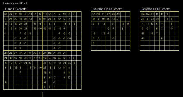
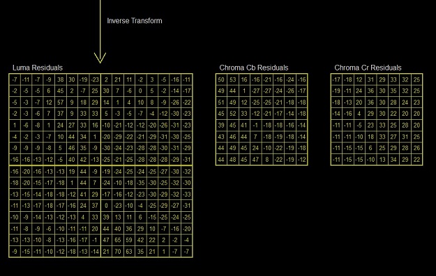
YUV mode allows the user to inspect the final decoded sample values, without additional overlay data.
Efficiency map mode gives a visual representation of how QP values are distributed in the image.
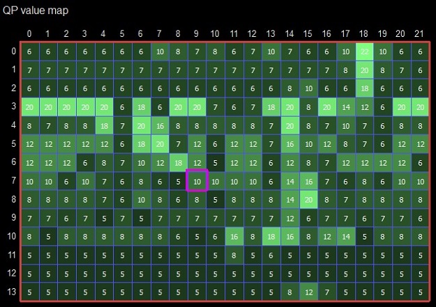
Simple Motion mode offers a way to quickly view the modes and motion of any picture at a glance. No overlays are present except a colored dot showing information about the PU's mode. Green dots indicate intra prediction, and purple/orange L0/L1 motion vectors for inter prediction are drawn as simple lines. When the motion vector is very small, a dot is drawn instead so that the mode is still easy to identify. When a motion vector does not point to the 0-th index of its respective list, the vector is drawn using a dashed line.
The following sections describe all available features when loading an AVC bitstream. The supported format of a bitstream is the raw bitstream with no surrounding container. Output from the publicly available AVC reference software JM is in this format and can be opened directly. VQ Analyzer supports profiles up to High profile. Sequences that go beyond the profile limits maybe be supported as well.
Use Mode menu to see available modes.
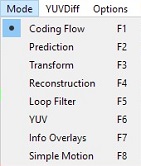
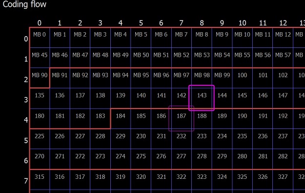
The coding flow mode gives a visual overview of the ordering of MBs in the stream, and some information of the decoding process. The blue grid shows the boundaries of the MBs in the picture. Each MB contains the MB address, which is simply the raster scan index of the CTB.
This mode shows the prediction units in each MB. MB splits are indicated with blue lines, which get darker as the split depth increases. When a MB split is implied by AVC (Direct mode for B slices) and not directly coded in the bitstream, the split lines are dashed.
Intra modes are indicated with green colors, and directional modes also show an arrow indicating the prediction direction. In the lower right corner of an intra MB the chroma mode is indicated in a darker green.
Inter Prediction units are indicated with cyan colors showing the Prediction unit splits and mode. Additionally, skipped blocks are shaded with a lined texture. The L0 motion vectors are drawn with an orange color, the L1 motion vectors (B slices only) are drawn with a purple color. The MV value is shown in the lower left corner along with the reference index.
Below is shown Prediction mode on a zoomed-in selection along the top edge of a picture. The selected MB is surrounded with a pink box while the selected Prediction Unit is surrounded with a yellow box.
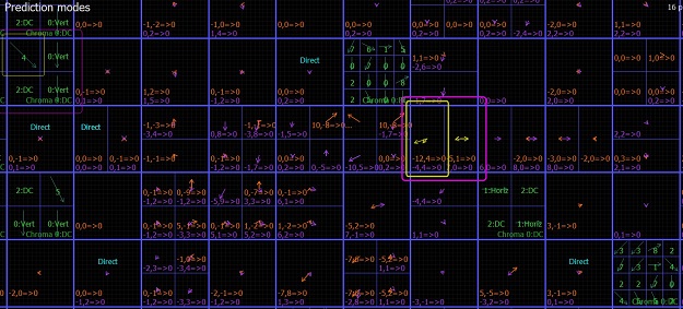
In Prediction mode, the sample values of a particular MB can be viewed in detail.
Intra MBs are displayed in green, and the left, upper-left and above prediction arrays are drawn adjacent.
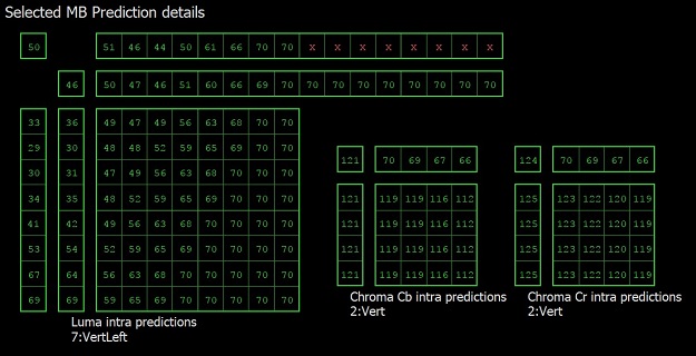
Inter MBs are displayed in cyan (turquoise).
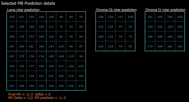
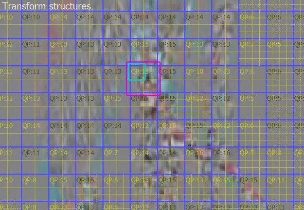
In Transform mode, the transforms and accompanying residual signal of the picture can be seen. As in Predictions mode, MB boundaries are shown with blue lines. The transform splits, when present, are indicated with yellow lines. QP values of each MB are shown in the upper-left corner. When this value is bright yellow, it means that a delta-QP was coded in the bitstream during the decode of that particular MB. Otherwise the number is dark. MBs that are PCM coded are marked with "PCM" in white.
If the "Pic" button is turned on, the raw residual signal is shown in image form. Residual values of 0 result in flat grey, negative values are darker and positive values are brighter.
Clicking on MBs causes that transform unit to be selected with a blue surrounding box. Clicking a transform unit repeatedly causes the selection to move up and cycle though the transforms in MB.
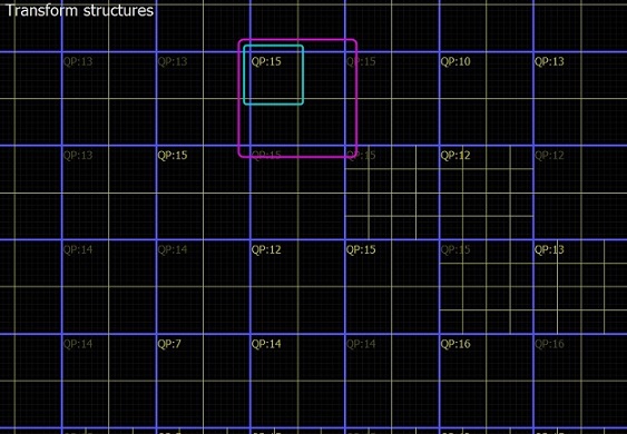
To view the full details of a particular MB, make the MB selection and enter detail mode by right clicking or using the detail mode button at the bottom of the main panel. In this mode the selected TU structure is drawn three times, arranged in a column from top to bottom, showing the 3 major steps in recovering the residual signal:
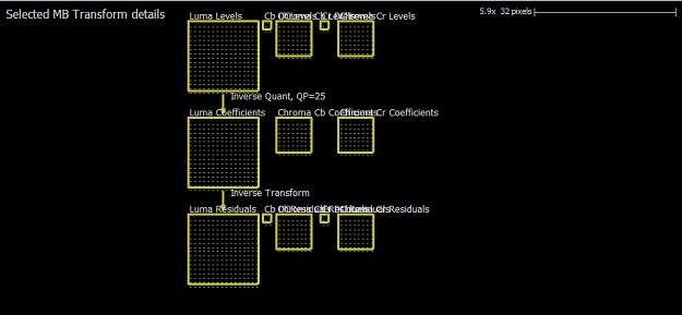
In Reconstruction mode, the reconstructed samples prior to deblocking can be inspected. As with Prediction/Transform mode, MB boundaries are shown with blue lines. MBs that have at least one transform with non-zero coefficients are marked with "Non-zero CBP". PCM-coded MBs are indicated with "PCM" in white.
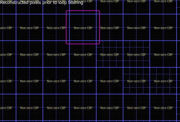
In detail mode, the reconstructed sample values can be inspected. The selection may be a single MB.
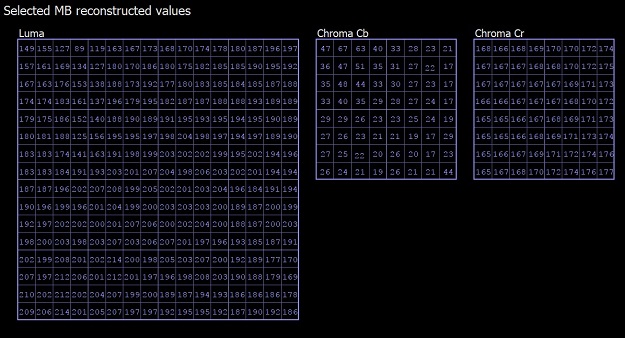
Loop Filter mode shows all edges processed by the deblocking filter.MB boundaries are not displayed in this mode, however MB selection still functions as in the other modes. Edges shown are for the luma deblocking process and are color coded in the following manner:
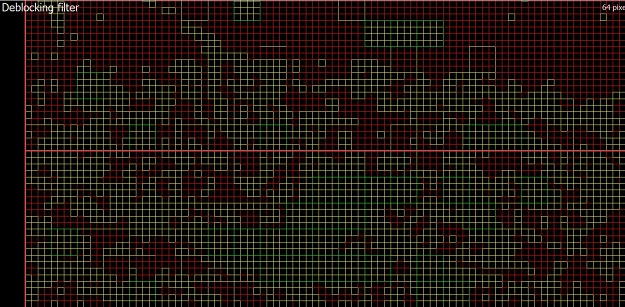
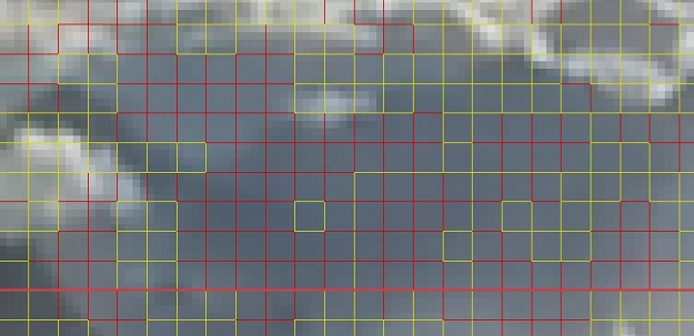
The deblocked sample values can be inspected directly in detail mode. As with Reconstruction Details, Sample values are indicated in yellow if they were modified by the deblocking process. Sample values that cannot be modified due to PCM MB or bypass_flag are indicated in red. Filtered edges belonging to the selected CU are shown in thick dashed lines, color coded the same way as in the non-detail mode. Each edge can be selected and clicked, bringing up a window showing the input values to the edge filter. Note that these values may differ from the reconstructed samples for horizontal edges, as they may have been modified by a vertical edge filter. Additionally, the boundary strength is displayed. Edges that were processed but ultimately not filtered (red colored) will indicate the reason. Typically, it is due to the boundary strength being 0, the threshold condition not being met, or a slice/tile edge when those edges shouldn't be processed.
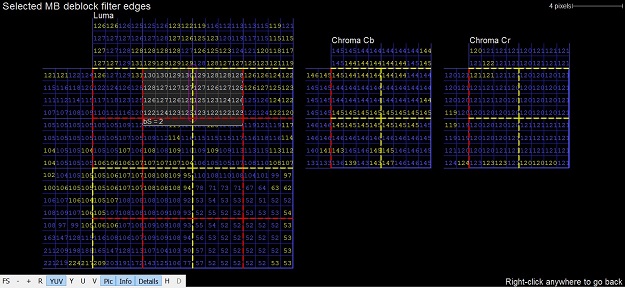
YUV mode allows the user to inspect the final decoded sample values, without additional overlay data.
There are a number of overlays that provide additional information about the picture that you're currently investigating. When you switch to "Info Overlays" mode, several additional submenus will appear in the bottom-left panel of info window.
You can switch now between additional modes with the drop down menu on the right. PSNR and SSIM modes are enabled if you have loaded a reference YUV file.
The heat map mode gives a visual representation of how the compressed bits of the picture are distributed spatially. Blocks with more bits per pixel are brighter than blocks with fewer. By zooming in, actual CU sizes in bits will be displayed as soon as its size is in the borders of the CU. By default, this mode also shows the CU quadtree boundaries in blue. It may be useful to turn off this overlay using the "Info" button on the lower left of the main panel. Heat Map does not offer a detail mode.
Maximum shown CU depth level can be restricted with the "Depth" on-screen control. Click on '+' and '-' to choose your required depth level.
The gradient used to display the heat map can also be edited:
The QP Map shows per-block QP. CUs with bigger QP are brighter than CUs with smaller QP. Coloring of the QP range can be adjusted with a gradient tool on the right top corner. On the 'skip' blocks, the QP does not change and they are colored red.
MB Type overlays show color map of their types. Intra blocks are colored in red, inter skips are yellow colored, B-Direct is in green and inter is in blue.
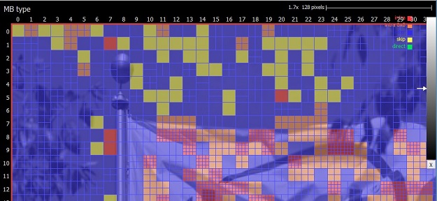
MB reference indices show reference indices for each subblock 8x8. Orange color shows L0 reference index and purple color is for L1 reference index. When PU has only one reference missing reference index is displayed with a dash. For blocks with no reference indices nothing is shown.
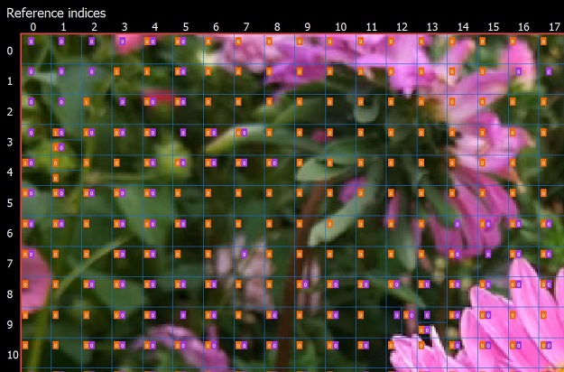
The PSNR map shows per-pixel PSNR values, normalized on block size. To enable this mode you have to load the reference YUV file via the DebugYUV menu. The value is calculated per block. A bigger value is shown with a brighter color. The color range can be adjusted with the gradient tool on the right top corner. If the block has no difference to the reference YUV, a letter 'e' is shown, standing for 'exact match'.
Simple Motion mode offers a way to quickly view the modes and motion of any picture at a glance. No overlays are present except a colored dot showing information about the PU's mode. Green dots indicate intra prediction, and purple/orange L0/L1 motion vectors for inter prediction are drawn as simple lines. When the motion vector is very small, a dot is drawn instead so that the mode is still easy to identify. When a motion vector does not point to the 0-th index of its respective list, the vector is drawn using a dashed line.
In the precinct mode picture is divided into blocks of 16*16 pixels. The blue grid shows block boundaries. Slice boundaries are shown with thick red lines. The selected block is highlighted with a pink square.
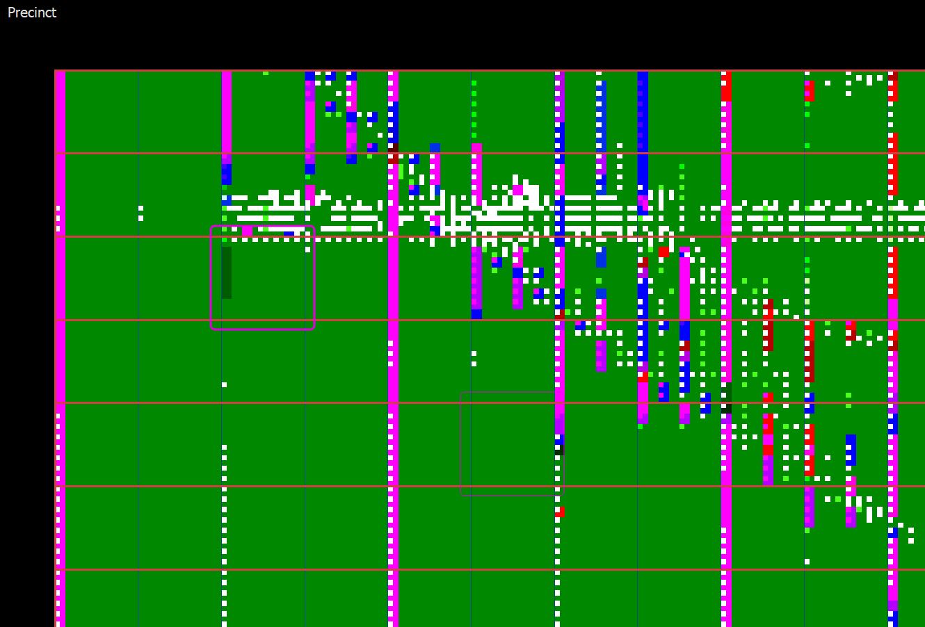
In the precinct details the quantized wavelet coefficients are shown for all components. By clicking on each coefficient, a pop-up appears with parameters related to this coefficient, such as precinct index, packets count, band and others, see screenshot.
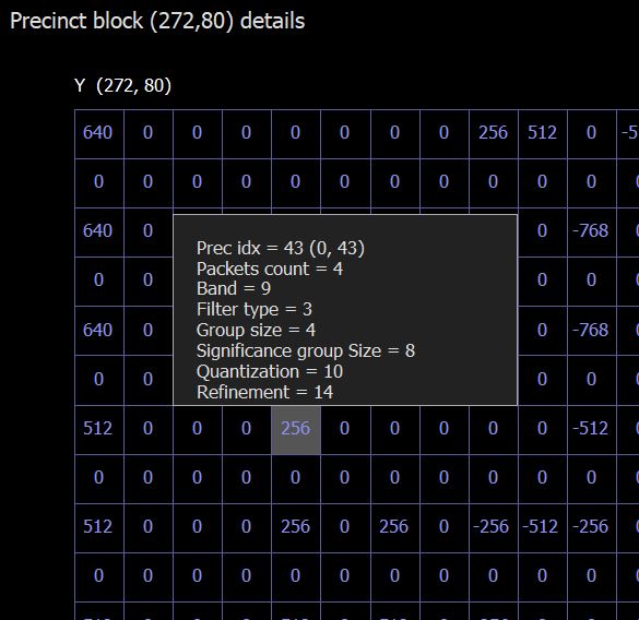
The preсinct tab shows the quantized wavelet coefficients of the precinct corresponding to the selected pixel. The coefficients are grouped by packets and coding groups. Сoefficients have different colors for each component. 1 component - white, 2 - blue, 3 - red, 4 if available - green.
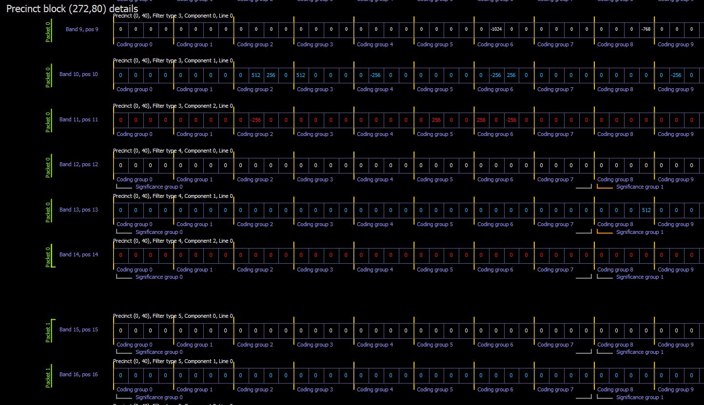
Each coefficient is clickable and the popup that appears shows the coordinates of this coefficient in the picture, as well as additional parameters.
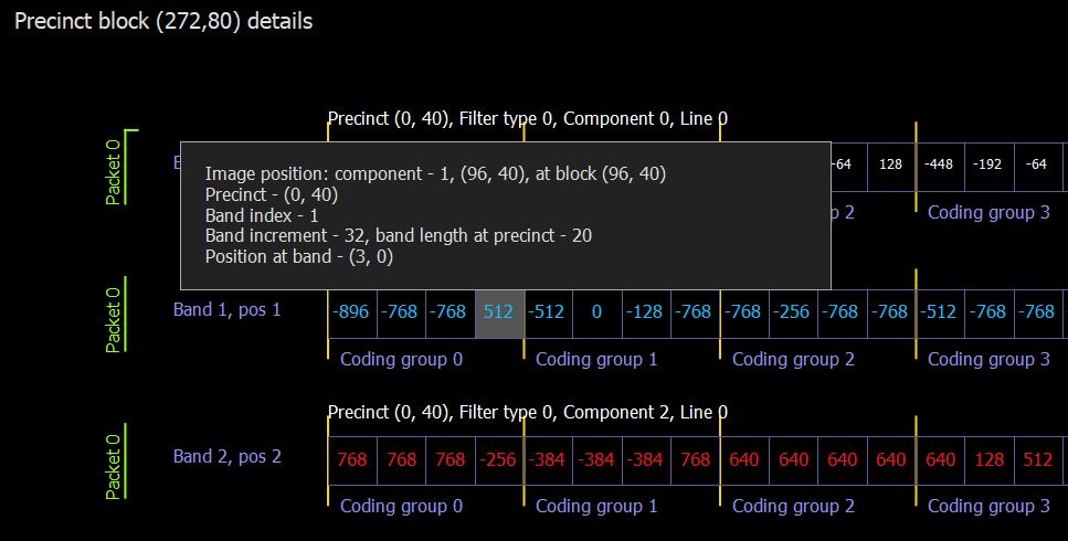
If JXS file has one vertical split, when the additional tab 'Precinct 1/2' is displayed in Precinct Details. The Precinct 1/2 tab displays bands and packets only from the top left corner of the image, with 1/2 width and 1/2 height.
If JXS file has two vertical splits, when two additional tabs 'Precinct 1/2' and 'Precinct 1/4' are displayed in Precinct Details. The Precinct 1/2 tab displays bands and packets only from the top left corner of the image, with 1/2 width and 1/2 height. The Precinct 1/4 tab displays bands and packets only from the top left corner of the image, with 1/4 width and 1/4 height.
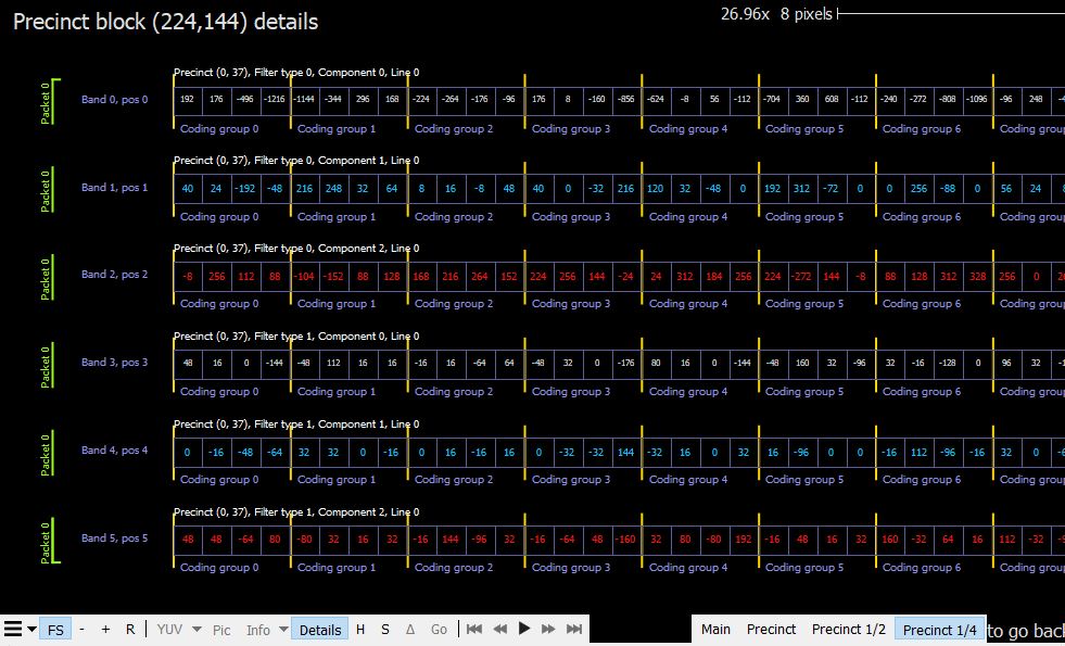
In the dequant mode picture is divided into blocks of 16*16 pixels. The blue grid shows block boundaries. Slice boundaries are shown with thick red lines. The selected block is highlighted with a pink square.
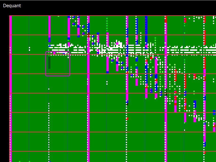
In the dequant details the wavelet coefficients after inverse quantization process are shown for all components. Below the block the type of the inverse quantization process is indicated (uniform or deadzone). By clicking on each coefficient, a pop-up appears. At the top of the popup the coordinates of the coefficient are indicated and at the bottom there are formulas and parameters for its calculation.
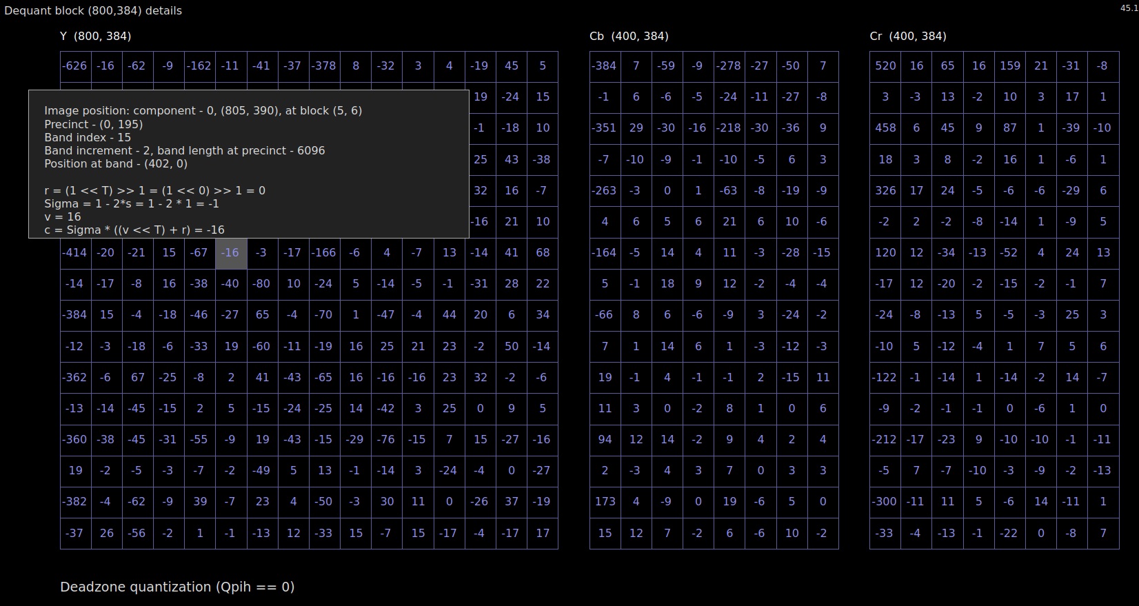
The dequant details also has a precinct tab where the coefficients are grouped by packets and coding groups. The popup in the precinct tab is the same as in the main dequant details.
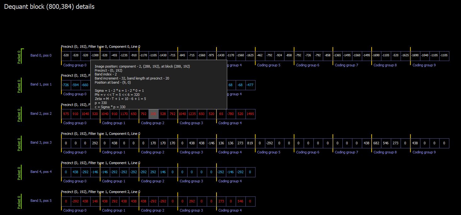
If JXS file has one vertical split, when the additional tab 'Precinct 1/2' is displayed in Dequant Details. The Precinct 1/2 tab displays bands and packets only from the top left corner of the image, with 1/2 width and 1/2 height.
If JXS file has two vertical splits, when two additional tabs 'Precinct 1/2' and 'Precinct 1/4' are displayed in Dequant Details. The Precinct 1/2 tab displays bands and packets only from the top left corner of the image, with 1/2 width and 1/2 height. The Precinct 1/4 tab displays bands and packets only from the top left corner of the image, with 1/4 width and 1/4 height.
In the transform mode picture is divided into blocks of 16*16 pixels. The blue grid shows block boundaries. The selected block is highlighted with a pink square.
In the transform details the inversely wavelet transformed sample values are shown for all components. Below the block the type of the inverse quantization process is indicated (uniform or deadzone). By clicking on each coefficient, a pop-up appears. At the popup the coordinates of the coefficient are indicated.
In the bands tab the inverse transformation stages are shown in detail.
If the value of the coefficient was changed during the inverse wavelet filtering process, it is colored yellow. By clicking on the yellow coefficient, the value of this coefficient at the previous stage of the inverse wavelet filtering process appears.
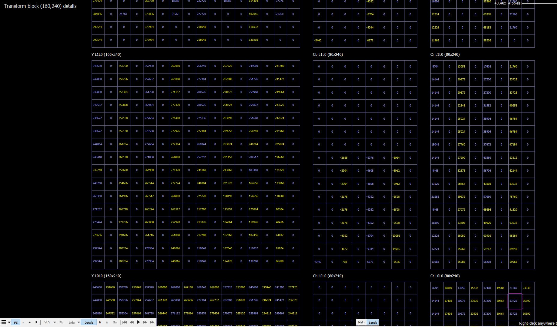
In the MCT mode picture is divided into blocks of 16*16 pixels. The blue grid shows block boundaries. The selected block is highlighted with a pink square.
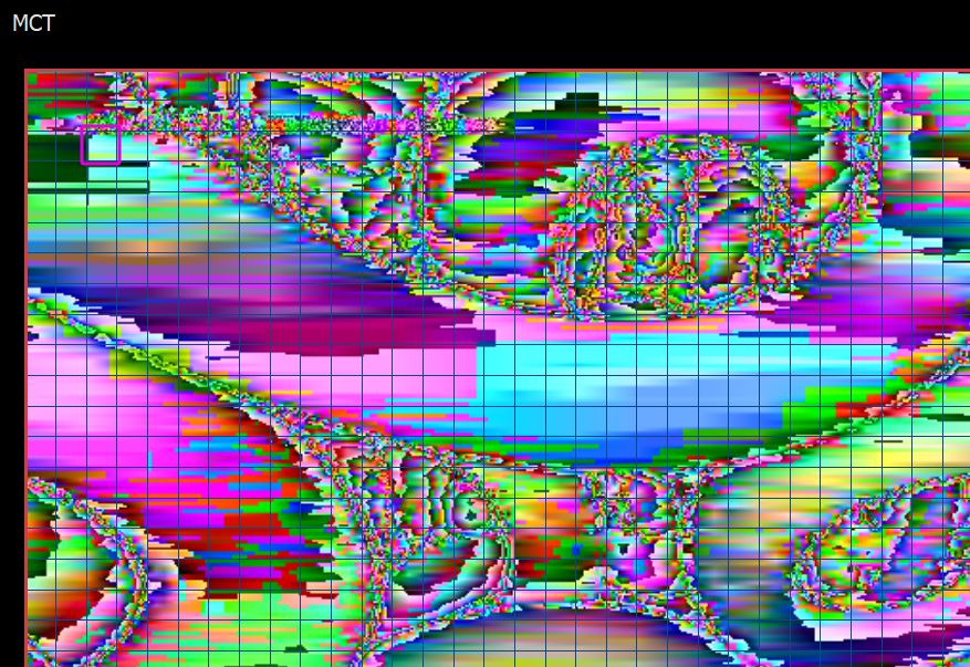
In the MCT details the sample values after the inverse multiple component transformation process are shown for all components. Below the block the type of the inverse multiple component transformation process is indicated.
If the inverse multiple component transformation is not used, NONE is written below the block and the sample values are the same as after inverse transformation.
In the case of the inverse reversible multiple component transformation, the sample values after inverse RCT are shown in detail. Each sample value is clickable and the parameters for its calculation are shown in the popup.
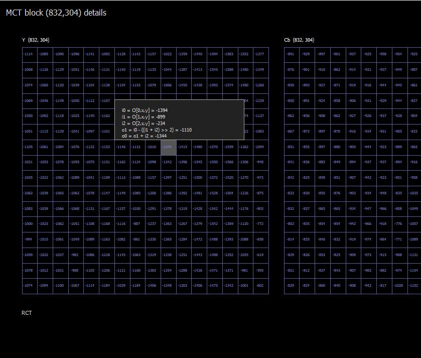
In the case of the inverse Star-Tetrix transformation, the sample values after inverse Star-Tetrix transformation are shown in detail. By clicking on the sample value, the popup with parameters and formulas of all steps of the Star-Tetrix transformation appears.
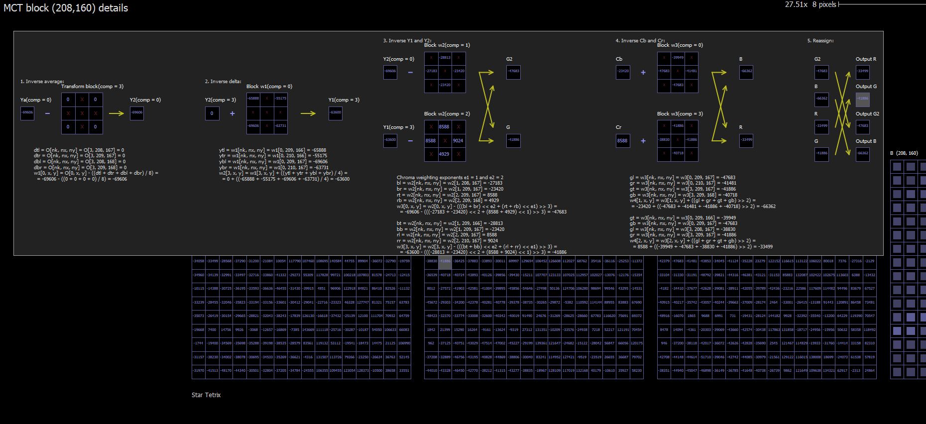
In the NLT mode picture is divided into blocks of 16*16 pixels. The blue grid shows block boundaries. The selected block is highlighted with a pink square.
In the NLT details the reconstructed sample values are shown for all components. By clicking on each coefficient, a pop-up appears. Calculations of output scaling and level shifting process are shown in popup.
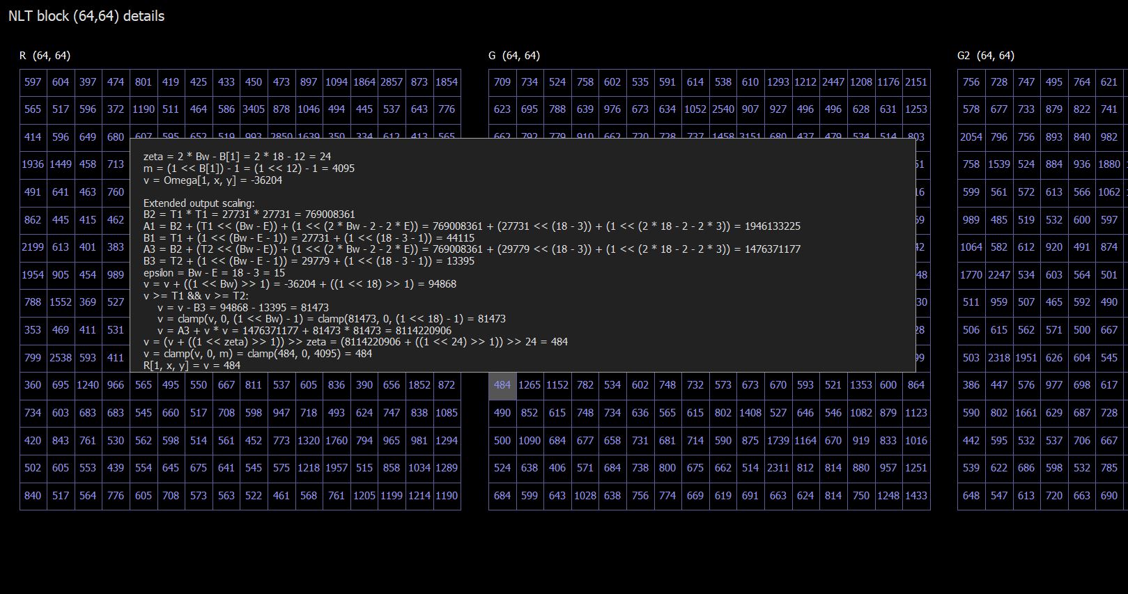
In the YUV mode picture is divided into blocks of 16*16 pixels. The blue grid shows block boundaries. The selected block is highlighted with a pink square.
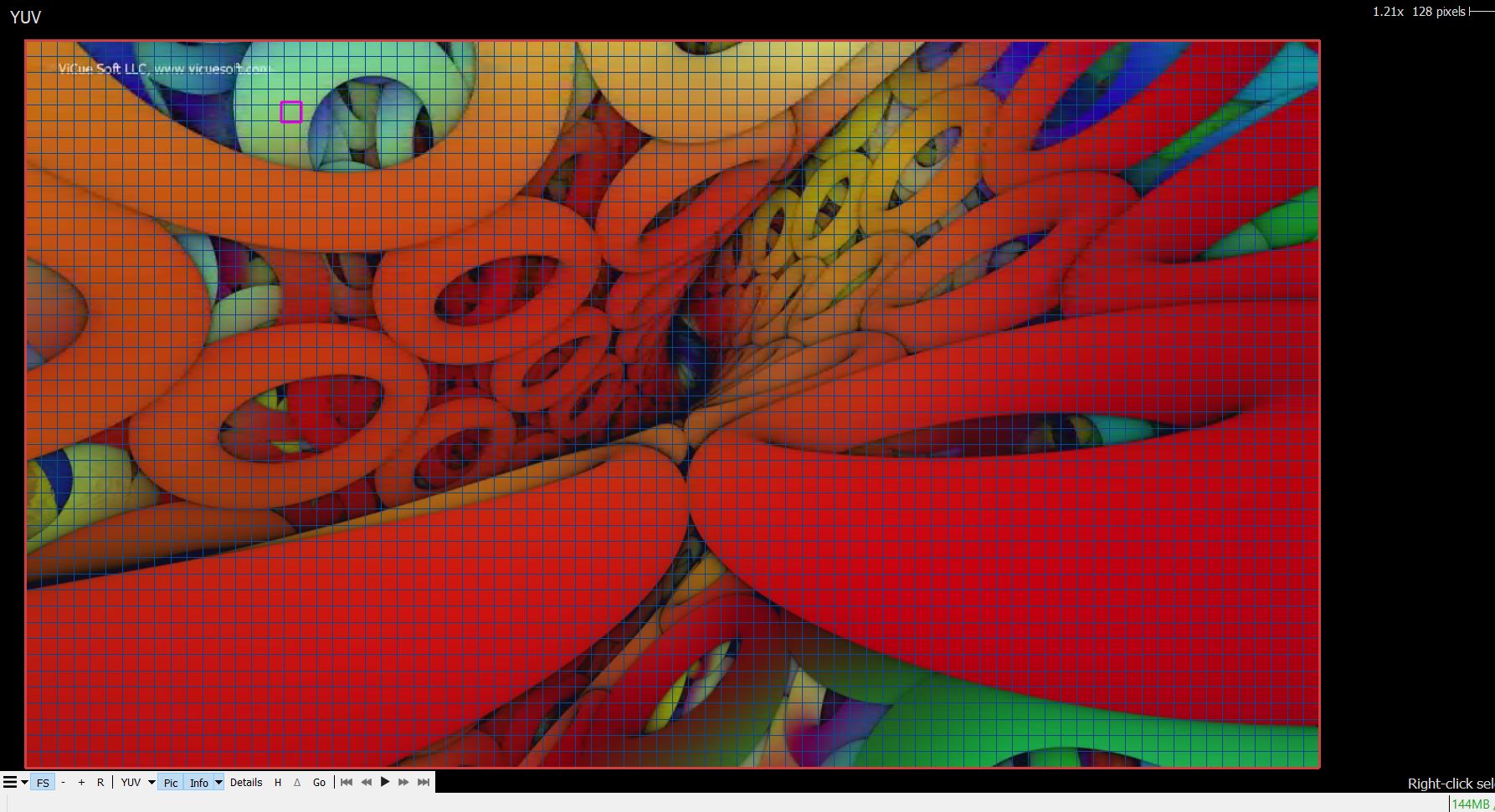
In the YUV details the final decoded sample values are shown for all components.
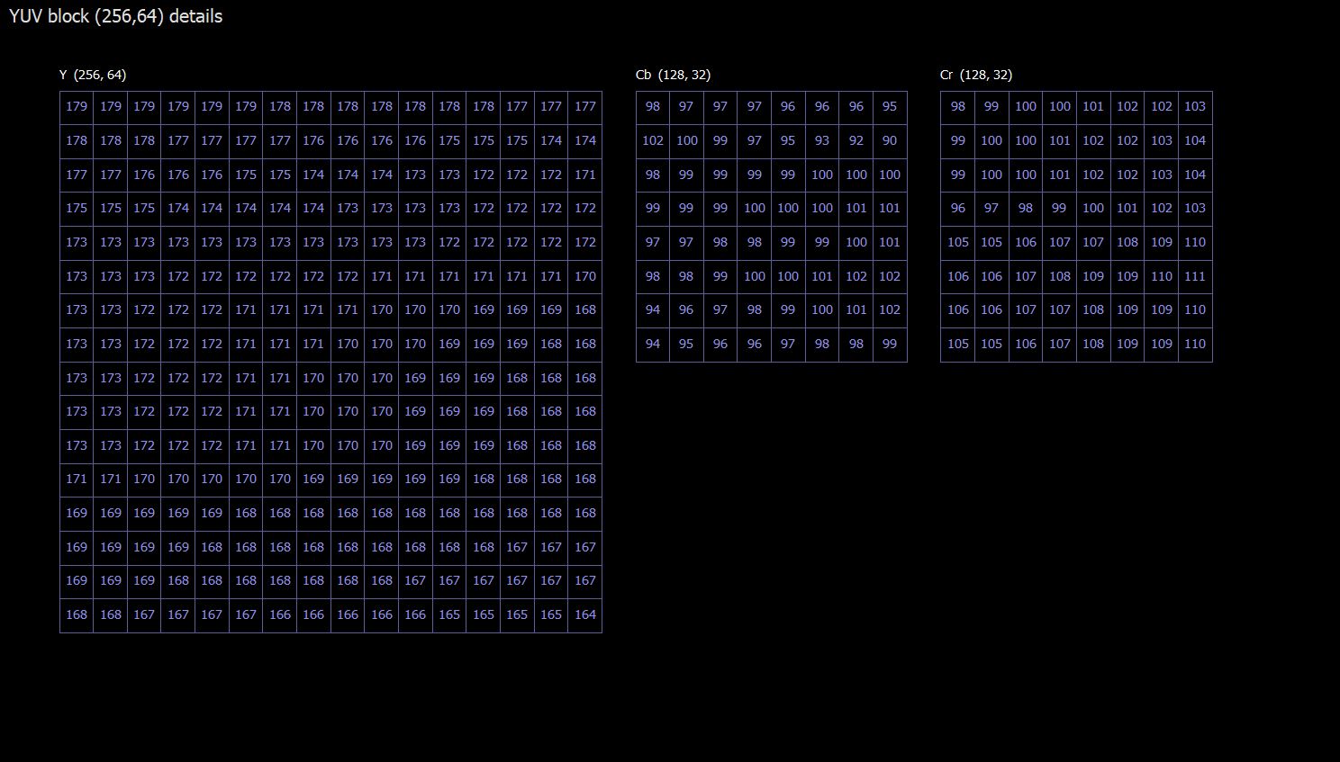
The following functions are available for all codecs.
Dual view mode allows one to make a direct visual comparison between two bitstreams. This feature is useful for fine tuning codecs with a slight variation in coding parameters. The bitstreams themselves should be coded with the same codec. VQ Analyzer considers the first opened stream to be the master stream. The depended stream is opened just after the master one by choosing "Open depended bitstream..." in File menu.
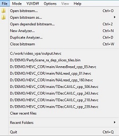
When the depended bitstream is opened it is synchronized with the master bitstream in frame position, chosen mode, offset and scaling factor in the central information window. Also, the toolbar buttons in central info window work synchronously with the master.
The VQ Analyzer provides a new delta button  in the toolbar of central window.
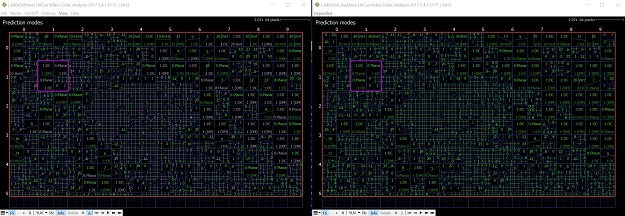
This button allows for a visual comparison between the master and depended bitstreams. When this mode is activated the blocks with the same structure and the same currently visualized modes will be in gray color, while the blocks with different parameters or blocks with different structure on both view still will be colored. In this way, it's simple for the user to see a visual difference in the coding parameters. The delta mode can be used for the following modes: Prediction, Transform, Reconstruction, Deblocking, SAO, Info overlays.
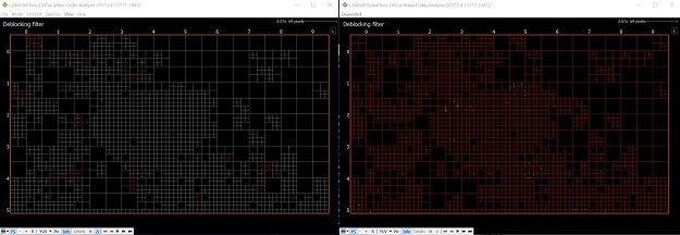
For heat map-like modes displaying one parameter, visual difference is shown pre block in three colors: red -- positive values, gray - zero difference, blue -- negative difference. So you can easily locate any increase or decrease in comparison with the depended bitstream.
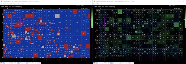
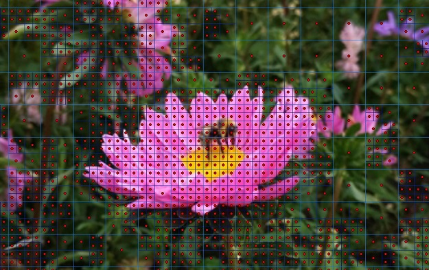
In YUV mode, the YUVDiff feature is exposed. This feature allows for comparison of an external decoded YUV file with the decoded bitstream. Supported formats are 4:2:0 planar and NV12. Also, YUV files that are zipped or gzipped may be opened directly without the need to decompress separately. If a zip file contains more than one YUV file, only the first one is used. When a YUV file is loaded, any mismatches will be indicated with a red dot in the CU containing the mismatch. This allows the user to quickly identify the nature of the mismatch which can assist with debugging.
When a file is opened, four additional buttons become visible on the lower left of the main window:

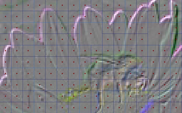
or absolute difference values, that is useful to identify particular pixels with difference.
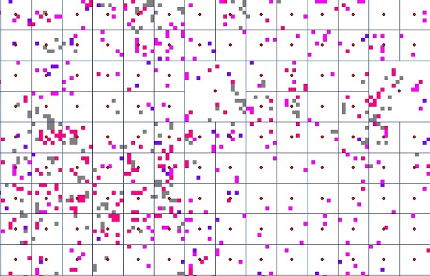
In detail mode, the expected YUV values can be inspected. Note that the displayed sample values are the same as those in the previous mode. When a YUV file is loaded, the debug and delta YUV values can be inspected as well. Mismatching values are shown in red.
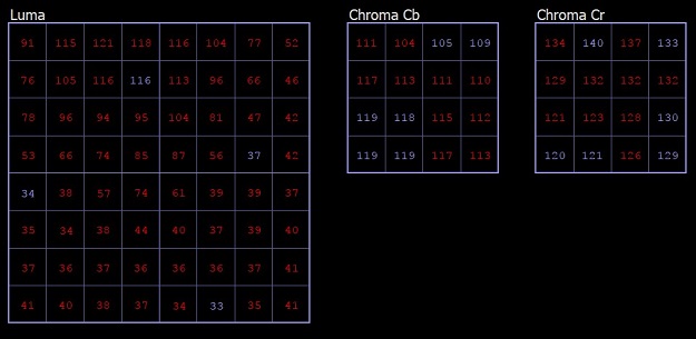
With "Diff YUV" button difference values switched on/off.
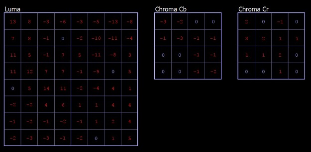
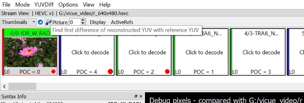
The feature "Find first difference of reconstructed YUV with reference YUV" works for all codecs VVC, AVS3, VP9, HEVC, AVC, MPEG2, AV1. By clicking the button with a magnifier icon, you can start a sequential search in decode order for the difference between the reconstructed YUV and the reference YUV that should be preloaded via YUVDiff menu. The search runs until the first difference is found or to the end of the stream. If you don't want to wait for the search to finish, the process can be cancelled at any time with the cancel button in the info modal dialog. The search always starts from the first picture in decoder order.
The following sections describe all available features when loading a YUV file. YUV allows the user to view different types of raw YUV data.
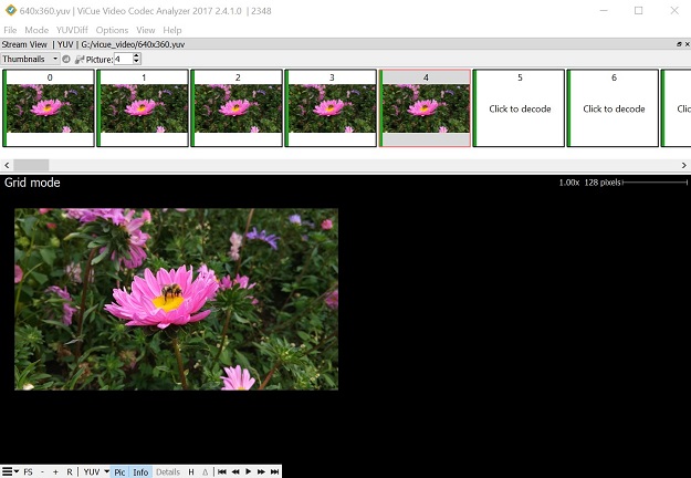
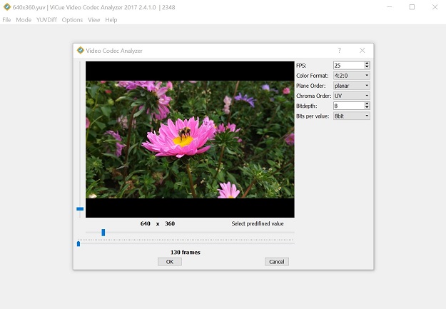
On loading a YUV file, the VQ Analyzer will try to guess the YUV width height and bitdepth based on file name and internal data. Files with special naming like file_widthxheight.yuv will skip internal sizes detection and use sizes from file name.
In any case, the VQ Analyzer will show a loading dialog for the YUV file to adjust loading parameters like width, height, chroma format, plane order, bitdepth, bits per value, and chroma order.
Width and Height labels are clickable. You can input values directly in it or use 'Select predifined value' combobox to select predifined values, or you can use the slider to choose sizes.
The bottom slider will change the frame and allows you to quickly and easily check the bitstream.
A few other features to keep in mind:
Qt licensed under the GNU Lesser General Public License (LGPL) version
Qwt
Qwt License Version 1.0, January 1, 2003
The Qwt library and included programs are provided under the terms of the GNU LESSER GENERAL PUBLIC LICENSE (LGPL) with the following exceptions:
The following example statement can be included in user documentation to satisfy this requirement: [program/widget] is based in part on the work of the Qwt project (<http://qwt.sf.net>).